Simulink OCP-solver S-function infeasible but Matlab equivalent OCP-solver feasible

Timdek · June 19, 2024, 3:34pm

Hi

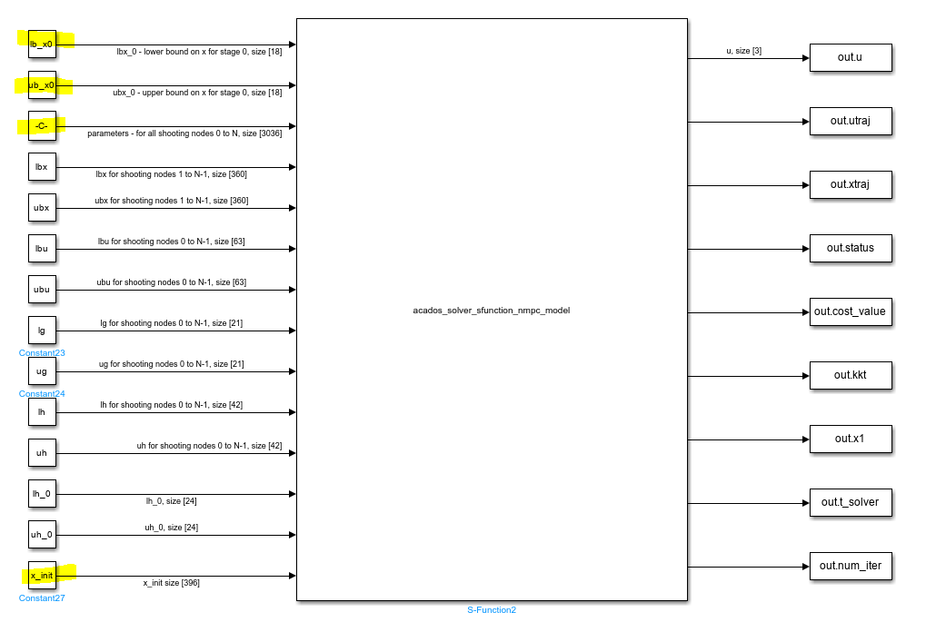
I am working on a NMPC model in ACADOS, via the MATLAB interface. I have created a model that runs smoothly in MATLAB. Now I want to export it to Simulink, but the performance there is very different. I created an S-function (ocp solver) from my MATLAB based model following the examples of simulink_example_advanced.m in the getting started folder. I used repmat to duplicate my inputs enough to fit the S-function input size requirements (as they are they required for the full horizon).

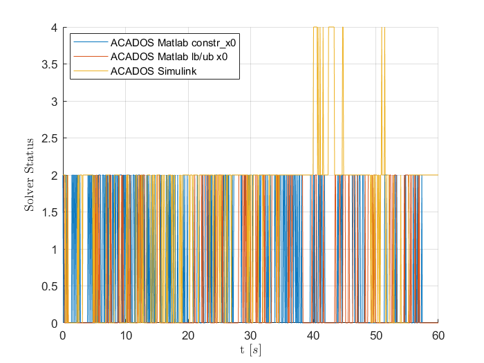
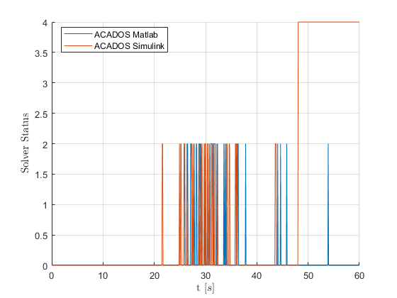
The Simulink based model returns different results over the full timeline (which is not necessarily problematic as long as they are ‘good enough’ as well), but more importantly becomes infeasible at a certain point in my simulation. This comparison is shown in the graph below (both models were evaluated with the same stopping criterion, all default except: nlp_solver_tol_stat 5e-3):

Solver_status_100it_comparison

If I were to make a guess at what is causing this, I would start with looking at the differences between the simulink based solver and the Matlab one. The only real difference between them is the fact that there is one option that I can not use in the Simulink model that I do have in my Matlab model. I use this option to progress my initial state in my next MPC evaluation, this is the option (it is placed within my for loop over my simulation time where I simulate my MPC use case):

ocp.set('constr_x0', xtraj(:,2)); % set the initial state

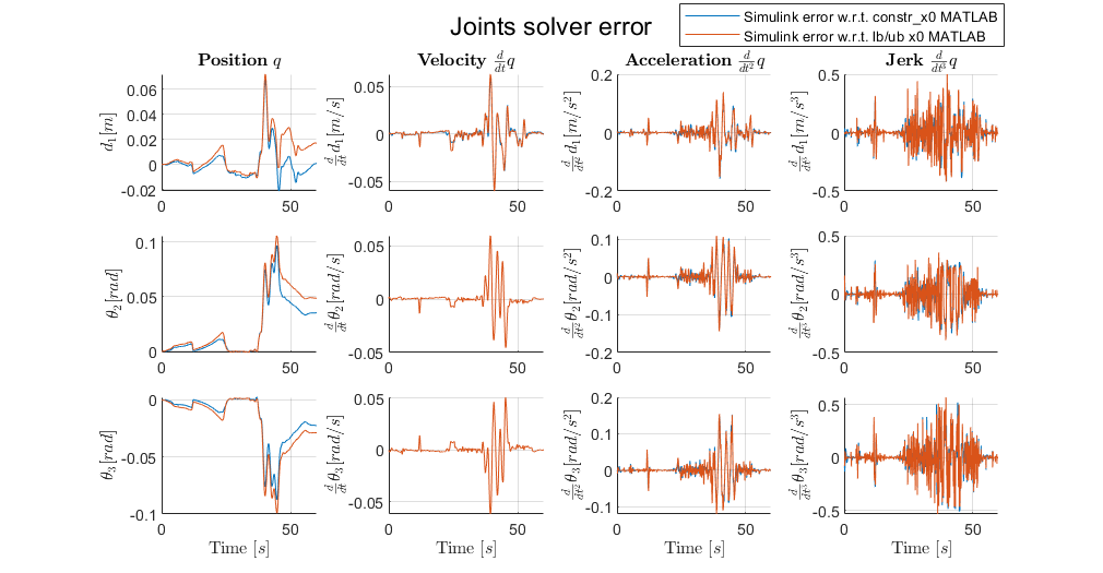
My solution to still have the same functionality in my simulink model was to than use the option lb_x0 and ub_x0 to constrain this initial state. I ran the MATLAB model with this change as well, and this model was still feasible at all solver calls. There was however a noteworthy difference in the chosen inputs that this model selected as opposed to that where I use the constr_x0 option. I believe this difference is because now that I set it as a constrain the state only needs to be that result within the constraint tolerances, (visible if I look at the x-trajectory, i.e. if I constrain a state as 0, it will result in a state being 1e-9). This difference is marginally and the states are generally very much alike, up until the approximately the point where in the Simulink solver the the solutions tend to start becoming infeasible. Hinting at that the root of the infeasibilities may lay at the difference in setting this option.

Do you perhaps know what the root is of the Simulink model resulting in all these infeasibilities?

Am I searching in the right direction with assuming it is caused by this absence of setting constr_x0?

p.s.

The only other potential root of the issue that I can think of is the setting of the S-function input lh_0 and uh_0. All constraints are defined as inputs for shooting nodes 0 to N-1 already in the other S-function inputs (lbx, ubx, lbu, ubu, lg,ug, lh, uh). So these feel like a duplicate input, or have I misunderstood how I should use these two S-function inputs.

Timdek · July 1, 2024, 7:28am

Is there someone who can help me answer this question?

FreyJo · July 1, 2024, 9:31am

Hi,

I would suggest to update as little data as possible when interacting with the Simulink solver.
I guess that you don’t need to update the bounds on u and for the nonlinear constraint h.

I used repmat to duplicate my inputs enough to fit the S-function input size requirements (as they are they required for the full horizon).

Here it sounds like you are using u_init. Is that the case?
Do you always initialize the u values also in your Matlab closed loop simulation?
I think that it is easy to do something differently in the initialization leading to the different behavior.

Best,
Jonathan

Timdek · July 1, 2024, 12:37pm

Hi Jonathan,

Thank you very much for your reply.

You are indeed correct that I am setting u_init. And you are also correct, that this is something that previously was not the case indeed. I have corrected this mistake, but it has not yet resolved the issue.

Maybe to provide more clarity here is the command window text after generating the S-function:

Successfully created sfunction:
acados_solver_sfunction_nmpc_model.mexw64

Note: Usage of Sfunction is as follows:
Inputs are:

lbx_0 - lower bound on x for stage 0, size [18]

ubx_0 - upper bound on x for stage 0, size [18]

parameters - concatenated for all shooting nodes 0 to N, size [3036]

lbx for shooting nodes 1 to N-1, size [360]

ubx for shooting nodes 1 to N-1, size [360]

lbu for shooting nodes 0 to N-1, size [63]

ubu for shooting nodes 0 to N-1, size [63]

lg for shooting nodes 0 to N-1, size [21]

ug for shooting nodes 0 to N-1, size [21]

lh for shooting nodes 0 to N-1, size [42]

uh for shooting nodes 0 to N-1, size [42]

lh_0, size [24]

uh_0, size [24]

initialization of x for all shooting nodes, size [396]

Outputs are:

u0, control input at node 0, size [3]

utraj, control input concatenated for nodes 0 to N-1, size [63]

xtraj, state concatenated for nodes 0 to N, size [396]

acados solver status (0 = SUCCESS)

cost function value

KKT residual

x1, state at node 1

CPU time

SQP iterations

This is the code I use to generate the S-Function:

simulink_opts = get_acados_simulink_opts;



simulink_opts.inputs.x_init = 1;
simulink_opts.inputs.u_init = 0;
simulink_opts.outputs.utraj = 1;
simulink_opts.outputs.xtraj = 1;
simulink_opts.outputs.cost_value = 1;

Create_solver_ACADOS;

%% Compile Sfunctions
cd c_generated_code
make_sfun; % ocp solver
make_sfun_sim; % integrator

The script Create_solver_ACADOS:


if ~exist('simulink_opts','var')
    disp('using acados simulink default options')
    simulink_opts = get_acados_simulink_opts;
    % simulink_opts.inputs.reset_solver = 1;
    simulink_opts.inputs.x_init = 1;
    simulink_opts.inputs.u_init = 0;
    % simulink_opts.inputs.constr_x0 =  1;
    
    simulink_opts.outputs.utraj = 1;
    simulink_opts.outputs.xtraj = 1;
    simulink_opts.outputs.cost_value = 1;
end

model_path = fullfile(pwd,'..','nmpc_model');
addpath(model_path)

check_acados_requirements()

%% solver settings
% N = 21; % number of discretization steps
T_predict = Ts*N; % [s] prediction horizon length
x0 = p.x_0; % initial state

nlp_solver = 'sqp'; % sqp, sqp_rti
qp_solver = 'partial_condensing_hpipm';
qp_solver_cond_N = 5; % condensing horizon (for partial condensing)
sim_method = 'irk'; % erk, irk, irk_gnsf

%% model dynamics
model = Define_NMPC_model_ACADOS(p, p_c); % dynamics, cost, constraints

%% acados ocp model
ocp_model = acados_ocp_model();
ocp_model.set('name', 'nmpc_model');
ocp_model.set('T', T_predict);  % prediction horizon

% symbolics
ocp_model.set('sym_x', model.sym_x);
ocp_model.set('sym_u', model.sym_u);
ocp_model.set('sym_p',model.sym_p);
ocp_model.set('sym_xdot', model.sym_xdot);

% cost
cost_type = 'ext_cost';  % auto, ext_cost, linear_ls
ocp_model.set('cost_type', cost_type);
ocp_model.set('cost_expr_ext_cost_0', model.cost_expr_ext_cost_0);
ocp_model.set('cost_expr_ext_cost', model.cost_expr_ext_cost);
ocp_model.set('cost_expr_ext_cost_e', model.cost_expr_ext_cost_e);


% dynamics
if (strcmp(sim_method, 'erk'))
    ocp_model.set('dyn_type', 'explicit');
    ocp_model.set('dyn_expr_f', model.dyn_expr_f_expl);
else % irk irk_gnsf
    ocp_model.set('dyn_type', 'implicit');
    ocp_model.set('dyn_expr_f', model.dyn_expr_f_impl);
end

% constraints (separate for initial, intermediate and terminal stages)
ocp_model.set('constr_type', 'auto');
ocp_model.set('constr_expr_h_0', model.constr_expr_h_0);
ocp_model.set('constr_expr_h', model.constr_expr_h);

lb_x                        = p.lb_x;
ub_x                        = p.ub_x;
lb_u                        = p.lb_u;
ub_u                        = p.ub_u;
lb_v                        = p.lb_v;
ub_v                        = p.ub_v;
lb_a                        = p.lb_a;
ub_a                        = p.ub_a;
lb_j                        = p.lb_j;
ub_j                        = p.ub_j;
ocp_model.set('constr_lh_0', [lb_x; lb_v; lb_u; lb_a; lb_j]); % lower bound on h
ocp_model.set('constr_uh_0', [ub_x; ub_v; ub_u; ub_a; ub_j]);  % upper bound on h
ocp_model.set('constr_lh', [lb_x; lb_v; lb_u; lb_a; lb_j]);
ocp_model.set('constr_uh', [ub_x; ub_v; ub_u; ub_a; ub_j]);

ocp_model.set('constr_x0', [x0; zeros(12,1)]);  % set the initial state

%% acados ocp options
ocp_opts = acados_ocp_opts();
ocp_opts.set('param_scheme_N', N);
ocp_opts.set('nlp_solver', nlp_solver);
ocp_opts.set('nlp_solver_max_iter',100);
ocp_opts.set('nlp_solver_tol_stat', 5e-3);
ocp_opts.set('sim_method', sim_method);

ocp_opts.set('ext_fun_compile_flags', ''); % '-O2'
ocp_opts.set('globalization', 'merit_backtracking') % turns on globalization



%% create ocp solver
ocp = acados_ocp(ocp_model, ocp_opts, simulink_opts);

The S-function in Simulink now looks like this:

I call this Simulink function multiple times within a for loop in a matlab script. All parameters that are highlighted can differ between calls in the for loop. All other parameters are set before the for loop and the first call and are not changed any more afterwards.

This means that indeed as you mention I do not require to update the bounds on u, and the non-linear constraint h. Should I then change the formulation and remove all non-highlighted parameters as an input parameter to the Simulink model?

The top two highlighted inputs are lb_x0 and ub_x0, these where constant in my original non-simulink script. But now they vary as I use them to constrain my initial shooting step position, as the option “constrain_x0” was no longer possible here (as explained in my original post).

Timdek · July 30, 2024, 8:01am

Is there somebody who has seen these types of problems when moving to Simulink from MATLAB before and/or can help me with this problem?

FreyJo · July 31, 2024, 9:38am

Hi Tim,

I understand that you test the solver in a closed-loop simulation in Simulink.
Do the trajectories match the ones of the corresponding MATLAB closed-loop simulation, at least until the point where one of the solvers returns non-zero status?
If so, the problem formulations do probably match and it might be an issue that comes from the different initializations.
I see in your screenshot that you have x_init in Simulink.
Do you also set all the corresponding values in MATLAB?

In order to initialize the solver only once in Simulink and subsequently ignore the initialization ports, you can use the recently added flag ignore_inits, added here Simulink interface: add initialization functionalities and tests by FreyJo · Pull Request #1158 · acados/acados · GitHub

I hope this helps fixing the issue!
Best,
Jonathan

Timdek · August 1, 2024, 3:51pm

Hi Jonathan,

Thank you so much for your continued support.

I am indeed using the ocp_solver s-function and not the integrator / sim s-function. I have not built my Simulink model to be a closed loop yet, as I first wanted to experiment with the basic functioning of the solver in Simulink for my problem, so instead I call it every timestep from MATLAB. But in MATLAB I have built the loop in such a way that the output states of the previous timestep the solver was called are indeed inputs for this timestep. Does that answer your question about closed-loop simulation?

The trajectories do not perfectly match those of the corresponding MATLAB simulation, although they are very close and only start to deviate significantly after the infeasible solutions start. Below a figure is attached which shows the difference in joint states between the MATLAB simulation where I used my original setting with “constr_x0” to ensure the continuation of the initial state, as well as with a corresponding MATLAB simulation where I do not use this “constr_x0” setting but instead constrain it via lb_x0 and ub_x0 similar to how it is done in Simulink.

The jerk (system input) and accelerations tend to differ a bit over the full simulation. Still, the joint positions start to vary significantly after the approximately 45-second mark where the infeasible solutions start.

I do set the x_init values in MATLAB. I do it as follows (where xtraj is the previous solution for the states): x_init = reshape(xtraj,[],1);.

Finally I downloaded the new version of acados and enabled the ignore_inits flag. I must admit that I do not fully understand it’s purpose, so for now, I just set it to 1 at all times as I believe this corresponded to ignoring the initialization ports. This did indeed improve the results as the solver is now no longer infeasible at all instances from the 45-second mark onward, it is however still frequently infeasible. The solver status over time is shown here:

(The image with the joint errors was created with this ignore_inits set to 1 in Simulink already)

Once again thanks for your answers to my questions. Although I do not fully understand what I just did with the ignore_inits flag, it improves the performance so your recommendations are steering me in the right direction.

I am unsure what is causing these remaining infeasibilities. I at least also tried it with the ignore inits flag being 0 at the first iteration and 1 afterwards but that did not help either.

Do you have an idea what could cause these remaining infeasible solutions in the Simulink output?

Thanks in advance!

Kind regards,

Tim