Hi,
I am currently working on implementing the following cost function for a nonlinear Model Predictive Control (NMPC) system. This function aims to address two simultaneous objectives:
- Minimizing tracking error while enforcing input rate constraints within the cost function.
- Maximizing the “F” information metric to enhance the vehicle’s state estimation in an unknown environment.
Cost function - Casadi implementation:
        xr = x_ref[0:12, :]
        x0 = x[0:12, :]
        cost = 0
        for k in range(self.horizon):
            cost += (X[0:12, k] - xr).T @ self.P @ (X[0:12, k] - xr)
            cost += (U[:, k + 1] - U[:, k]).T @ self.R @ (U[:, k + 1] - U[:, k])
            cost += -alpha * F

            opt.subject_to(
                X[:, k + 1]
                == self.forward_dynamics(
                    X[:, k], U[:, k], flow_bf, flow_acc_bf, self.model_type
                )
            )
            opt.subject_to(opt.bounded(self.xmin, X[0:12, k], self.xmax))
            opt.subject_to(opt.bounded(self.umin, U[:, k], self.umax))

        cost += (X[0:12, -1] - xr).T @ self.P @ (X[0:12, -1] - xr)

        opt.subject_to(opt.bounded(self.xmin, X[0:12, -1], self.xmax))
        opt.subject_to(X[0:12, 0] == X0)

        opt.set_value(X0, x0)
I have successfully implemented the mentioned formulation using CasADi, and it performs well. However, the computation time is relatively high. Consequently, I’ve decided to switch to using acados with a Python interface to potentially improve efficiency.
As an initial step, I’ve broken down the problem and opted to implement only a portion of it, focusing solely on minimizing tracking error:
Reduced cost function - Casadi implementation:
        xr = x_ref[0:12, :]
        x0 = x[0:12, :]
        cost = 0
        for k in range(self.horizon):
            cost += (X[0:12, k] - xr).T @ self.P @ (X[0:12, k] - xr)
            cost += (U[:, k + 1] - U[:, k]).T @ self.R @ (U[:, k + 1] - U[:, k])

            opt.subject_to(
                X[:, k + 1]
                == self.forward_dynamics(
                    X[:, k], U[:, k], flow_bf, flow_acc_bf, self.model_type
                )
            )
            opt.subject_to(opt.bounded(self.xmin, X[0:12, k], self.xmax))
            opt.subject_to(opt.bounded(self.umin, U[:, k], self.umax))

        cost += (X[0:12, -1] - xr).T @ self.P @ (X[0:12, -1] - xr)

        opt.subject_to(opt.bounded(self.xmin, X[0:12, -1], self.xmax))
        opt.subject_to(X[0:12, 0] == X0)

        opt.set_value(X0, x0)
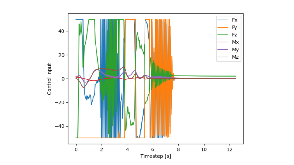
However, I’ve encountered difficulties defining (u_{k+1} - u{k}).T * R * (u_{k+1} - u{k}) when using “NONLINEAR_LS”. This has resulted in discontinuous output from the optimizer, as illustrated in the figure below:
I would greatly appreciate guidance on how to implement this using the “EXTERNAL” cost type, as I haven’t found any examples addressing a similar challenge.
I’ve attached the acados implementation that produces the discontinuous output as shown above:
model:
    def auv_model(self):
        x = SX.sym("x", (12, 1))
        x_dot = SX.sym("x_dot", (12, 1))
        u = SX.sym("u", (self.thrusters, 1))

        f_expl_expr = self.nonlinear_dynamics(x, u, self.model_type)
        f_impl_expr = x_dot - f_expl_expr

        p = []

        self.acados_model.name = "bluerov2"
        self.acados_model.f_expl_expr = f_expl_expr
        self.acados_model.f_impl_expr = f_impl_expr
        self.acados_model.x = x
        self.acados_model.xdot = x_dot
        self.acados_model.u = u
        self.acados_model.p = p
solver description:
    def create_ocp_solver_description(self):
        self.acados_ocp.model = self.acados_model
        x = self.acados_model.x
        nx = self.acados_model.x.shape[0]
        nu = self.acados_model.u.shape[0]
        self.acados_ocp.dims.N = self.horizon

        self.acados_ocp.cost.cost_type = "NONLINEAR_LS"
        self.acados_ocp.cost.cost_type_e = "NONLINEAR_LS"
        self.acados_ocp.cost.W_e = self.P
        self.acados_ocp.cost.W = self.P
        self.acados_ocp.model.cost_y_expr = x
        self.acados_ocp.model.cost_y_expr_e = x
        self.acados_ocp.cost.yref = np.zeros((nx,))
        self.acados_ocp.cost.yref_e = np.zeros((nx,))

        self.acados_ocp.constraints.lbu = self.umin
        self.acados_ocp.constraints.ubu = self.umax
        self.acados_ocp.constraints.lbx = self.xmin
        self.acados_ocp.constraints.ubx = self.xmax
        self.acados_ocp.constraints.lbx_0 = self.xmin
        self.acados_ocp.constraints.ubx_0 = self.xmax
        self.acados_ocp.constraints.idxbu = np.arange(nu)
        self.acados_ocp.constraints.idxbx = np.arange(nx)
        self.acados_ocp.constraints.idxbx_0 = np.arange(nx)

        # set options

        # self.acados_ocp.solver_options.qp_solver = "PARTIAL_CONDENSING_HPIPM"
        self.acados_ocp.solver_options.qp_solver = "FULL_CONDENSING_QPOASES"
        # self.acados_ocp.solver_options.qp_solver = "PARTIAL_CONDENSING_OSQP"
        self.acados_ocp.solver_options.qp_solver_cond_N = self.horizon
        self.acados_ocp.solver_options.hessian_approx = (
            "GAUSS_NEWTON"  # 'GAUSS_NEWTON', 'EXACT'
        )
        self.acados_ocp.solver_options.integrator_type = "IRK"
        self.acados_ocp.solver_options.sim_method_num_stages = 4
        self.acados_ocp.solver_options.sim_method_num_steps = 1
        self.acados_ocp.solver_options.nlp_solver_type = "SQP"  # SQP_RTI, SQP
        self.acados_ocp.solver_options.nlp_solver_max_iter = 500
        self.acados_ocp.solver_options.levenberg_marquardt = 1e-5
        self.acados_ocp.solver_options.tf = self.T_horizon
optimize:
def optimize(self, x, x_ref):
        xr = x_ref[0:12, :]
        x0 = x[0:12, :]
        N = self.horizon

        nx = self.acados_ocp.model.x.shape[0]
        nu = self.acados_ocp.model.u.shape[0]

        # initialize solver
        for stage in range(N + 1):
            self.acados_ocp_solver.set(stage, "x", np.zeros((nx,)))
        for stage in range(N):
            self.acados_ocp_solver.set(stage, "u", np.zeros((nu,)))

        # set initial state constraint
        self.acados_ocp_solver.set(0, "lbx", x0)
        self.acados_ocp_solver.set(0, "ubx", x0)

        for k in range(N):
            self.acados_ocp_solver.set(k, "yref", xr)
        self.acados_ocp_solver.set(N, "yref", xr)

        status = self.acados_ocp_solver.solve()
        if status != 0:
            print("acados returned status {}".format(status))

        force_axes = self.acados_ocp_solver.get(0, "u")
        # self.previous_control = np.array([force_axes]).T

        u_next = evalf(mtimes(pinv(self.auv.tam), force_axes)).full()

        return force_axes, u_next
Any assistance would be greatly appreciated! Thank you!