Hello,
I am working on a nonlinear model predictive control (NMPC) problem for a racing car using the Matlab interface of Acados. The goal is to control the racing car to follow a given trajectory while minimizing control effort. The trajectory optimization also using Acados solver and successfull. I’m using the below model:
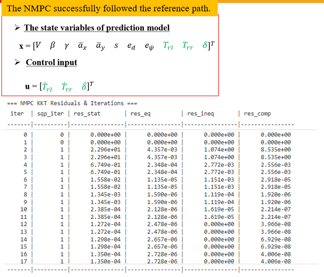
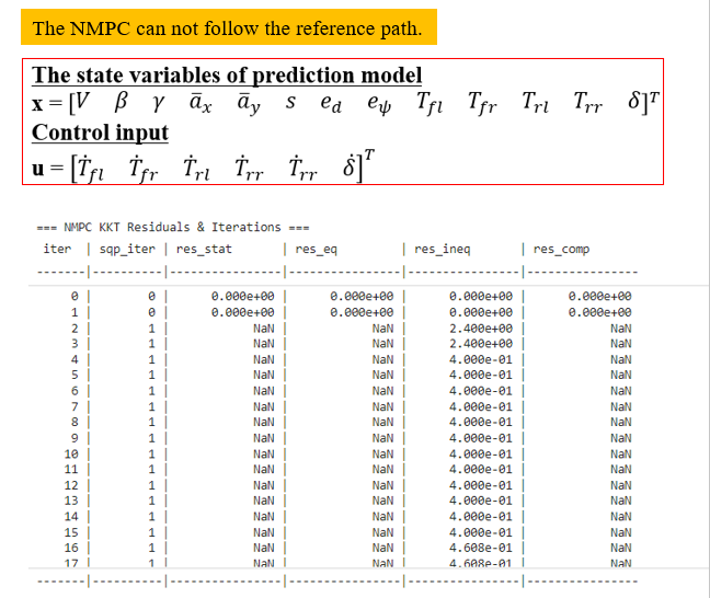
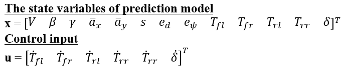
The state variables of prediction model
I am encountering three main issues during the simulation:
-
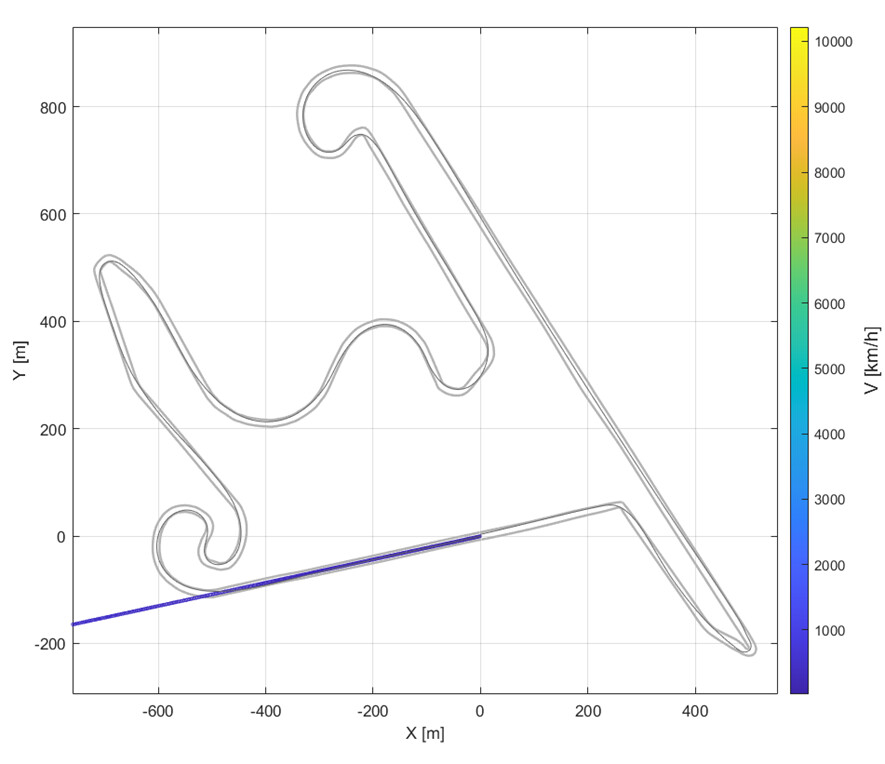
Trajectory tracking: The vehicle does not follow the reference trajectory properly – it cuts corners significantly, especially in tight turns (see attached figure: gray = reference, blue = actual, color = speed).
-
Cost function: Please reference to the below code
%% COST FUNCTION

eV_max = 1;

ebeta_max = 0.05;

n_max = 0.1;

chi_max = 0.05;

beta_ref = atan(delta*veh.lr/veh.l);

symx = vertcat((beta-beta_ref)/ebeta_max, (V-V_ref)/eV_max, n/n_max, chi/chi_max);

symu = vertcat(dot_Tfl/dot_Tfl_s, dot_Tfr/dot_Tfr_s,dot_Trl/dot_Trl_s, dot_Trr/dot_Trr_s, dot_delta/dot_delta_s);

Q = diag([1, 1, 100, 100]);

R = diag([1, 1, 1, 1, 1]);

delta_ff = atan(veh.l * kappa);

% (1) Track curvature feedforward

J_delta_ff = 2 * (delta - delta_ff)^2;

% (2) Frenet feedback (force convergence to centerline)

J_delta_fb = 5 * (delta - delta_ff - 0.8*n - 0.5*xi)^2;

% -------- Torque vectoring penalties (LIGHT) --------

LR = (Tfl - Tfr)^2 + (Trl - Trr)^2;

FB = ((Tfl + Tfr) - (Trl + Trr))^2;

Mz_drive = veh.wt/(2*veh.rw) * ( (Tfr - Tfl) + (Trr - Trl) );

Yaw_term = Mz_drive^2;

% -------- Stage cost --------

model.expr_ext_cost = ...

0.5 * (symx.' * Q * symx) ...

+ 0.5 * (symu.' * R * symu) ...

+ J_delta_ff ...

+ J_delta_fb ...

+ 0.0005 * LR ...

+ 0.001 * FB ...

+ 0.001 * Yaw_term;

model.expr_ext_cost_e = 0.5*symx'*Q*symx;


3. NMPC generate: Please reference to the below code

```matlab
% 4WD NMPC – ACADOS Codegen

% Matching new ocp_model_racecar_4wd (13 states, 5 inputs)

clear all; clc;

if ~isdeployed

cd(fileparts(which('nmpc_gen')));

end

if isfile('c_generated_code\CMakeCache.txt')

delete('c_generated_code\CMakeCache.txt');

end

acados_env_variables_windows

%% Vehicle parameters, initial conditions

veh = veh_params();

opt_e = 1e-3;

V0 = 5; % initial speed

%% Load model (13-state 4WD)

model = ocp_model_racecar();

nx = model.nx;

nu = model.nu;

np = model.np;

x_s = model.x_s;

u_s = model.u_s;

N = model.N;

T = model.T;

Ts = model.Ts;

%% Create OCP model

ocp_model = acados_ocp_model();

ocp_model.set('name', model.name);

ocp_model.set('T', model.T);

ocp_model.set('sym_x', model.x);

ocp_model.set('sym_xdot', model.xdot);

ocp_model.set('sym_u', model.u);

ocp_model.set('sym_p', model.p);

%% Dynamics: IRK

sim_method = 'irk';

%Dynamics

if (strcmp(sim_method,'erk'))

ocp_model.set('dyn_type', 'explicit');

ocp_model.set('dyn_expr_f', model.expr_f_expl);

elseif (strcmp(sim_method, 'irk'))

ocp_model.set('dyn_type', 'implicit');

ocp_model.set('dyn_expr_f', model.expr_f_impl);

end

%% Cost function

ocp_model.set('cost_type', 'ext_cost');

ocp_model.set('cost_type_e', 'ext_cost');

ocp_model.set('cost_expr_ext_cost', model.expr_ext_cost);

ocp_model.set('cost_expr_ext_cost_e', model.expr_ext_cost_e);

ny_x = 4;

ny_e = ny_x;

ny_u = 5;

ny = ny_x + ny_u;

nbx = nx;

Jbx = eye(nx);

ocp_model.set('constr_Jbx', Jbx);

ocp_model.set('constr_lbx', model.x_min);

ocp_model.set('constr_ubx', model.x_max);

%% Input bounds (5)

nbu = 5;

Jbu = eye(nbu,nu);

ocp_model.set('constr_Jbu', Jbu);

ocp_model.set('constr_lbu', model.u_min);

ocp_model.set('constr_ubu', model.u_max);

% Nonlinear constraints: 5 inequalities (μ ellipse + orthogonality)

nh = 5;

ocp_model.set('constr_expr_h', model.constraint.expr);

ocp_model.set('constr_lh', [0, 0, 0, 0, 0]);

ocp_model.set('constr_uh', [0, 1, 1, 1, 1]);

Jsh = eye(nh);

ocp_model.set('constr_Jsh', Jsh);

ocp_model.set('cost_zl', zeros(nh,1));

ocp_model.set('cost_zu', zeros(nh,1));

ocp_model.set('cost_Zl', diag([10 10 10 10 1]));

ocp_model.set('cost_Zu', diag([10 10 10 10 1]));


% Initial state for solver (13 states)

x0 = zeros(nx,1);

x0(9) = 5; % Tfl

x0(10) = 5; % Tfr

x0(11) = 5; % Trl

x0(12) = 5; % Trr

%x0(13) = 0; % delta

x0 = x0 ./ model.x_s; % normalize

ocp_model.set('constr_x0', x0);

%% Solver parameters

compile_interface = 'auto';

codgen_model = 'true';

nlp_solver = 'sqp_rti'; % sqp, sqp_rti

% nlp_solver = 'sqp_rti'; % sqp, sqp_rti

qp_solver = 'full_condensing_hpipm'; % full_condensing_hpipm, partial_condensing_hpipm, full_condensing_qpoases

nlp_solver_exact_hessian = 'true'; % false=gauss_newton, true=exact


%% acados ocp set opts

ocp_opts = acados_ocp_opts();

ocp_opts.set('compile_interface', compile_interface);

ocp_opts.set('codgen_model', codgen_model);

ocp_opts.set('param_scheme_N', model.N);

ocp_opts.set('nlp_solver', nlp_solver);

ocp_opts.set('nlp_solver_exact_hessian', nlp_solver_exact_hessian);

ocp_opts.set('sim_method', sim_method);

ocp_opts.set('sim_method_num_stages', 2);

ocp_opts.set('sim_method_num_steps', 1)

ocp_opts.set('qp_solver', qp_solver);

% nlp solver

eps_nlp = 1e-4;

ocp_opts.set('nlp_solver_max_iter', 30);

ocp_opts.set('nlp_solver_tol_stat', eps_nlp);

ocp_opts.set('nlp_solver_tol_eq', eps_nlp);

ocp_opts.set('nlp_solver_tol_ineq', eps_nlp);

ocp_opts.set('nlp_solver_tol_comp', eps_nlp);

% ... see ocp_opts.opts_struct to see what other fields can be set

p0 = [5, V0];

ocp_opts.set('parameter_values', p0);

%% get available simulink_opts with default options

simulink_opts = get_acados_simulink_opts;

% manipulate simulink_opts

% inputs

simulink_opts.inputs.lbx = 1;

simulink_opts.inputs.ubx = 1;

simulink_opts.inputs.lh = 0;

simulink_opts.inputs.uh = 0;

simulink_opts.inputs.lbu = 0;

simulink_opts.inputs.ubu = 0;

% outputs

simulink_opts.outputs.utraj = 1;

simulink_opts.outputs.xtraj = 1;

simulink_opts.outputs.cost_value = 1;

simulink_opts.outputs.KKT_residual = 0;

simulink_opts.outputs.KKT_residuals = 1;

%% Generate acados OCP

ocp = acados_ocp(ocp_model, ocp_opts, simulink_opts);

%% set initial trajectory

x_init = zeros(N+1,nx);

x_init(:,1) = V0*ones(N+1,1);

x_init(:,9) = opt_e*ones(N+1,1);

x_init(:,10) = opt_e*ones(N+1,1);

x_init(:,11) = opt_e*ones(N+1,1);

x_init(:,12) = opt_e*ones(N+1,1);

x_init = x_init./model.x_s';

u_init = zeros(N,nu);

ocp.set('init_x', x_init');

ocp.set('init_u', u_init');

ocp.set('init_pi', zeros(nx, N));

%% Compile Sfunctions

cd c_generated_code

make_sfun; % ocp solver

% make_sfun_sim; % integrator

copyfile('acados_solver_sfunction_nmpc.mexw64','..\sim')

cd ..\sim
What I have checked/tried:
- Reference trajectory is correctly interpolated and updated at every MPC step.
- Cost function weights have been tuned (tracking weights increased significantly).
- Control inputs and states are updated correctly in the loop.
- No obvious mismatches in dimensions or scaling.
Question: - Any common pitfalls in Acados setup that lead to corner-cutting?
- Are there any configuration issues in my OCP setup that could cause these problems?
- What steps should I take to improve the trajectory tracking and ensure the cost function reflects the error properly?