Accessing inputs from other shooting steps and setting the parameter vector for individual shooting steps

Hi :wave:

I am currently converting my NMPC that was formulated in casadi to acados using the matlab interface, as ACADOS offers code generation and simulink support via the S-Functions. Which is great! So thanks for this great tool!

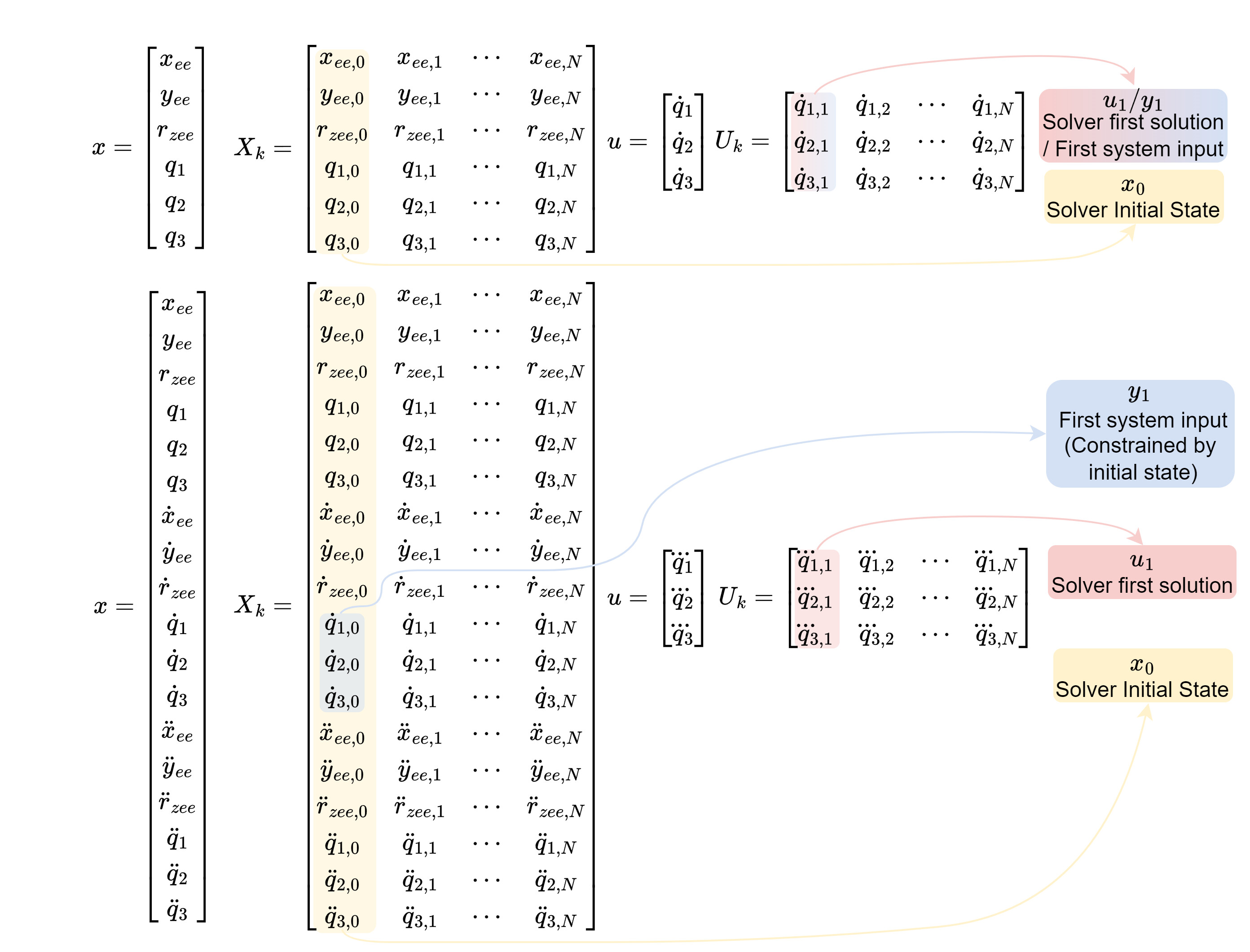
In my casadi implementation my optimization variables where my states and inputs over my prediction horizon N. So for example say my system (in simplified version) is described like this:

x = \begin{bmatrix} q_1 \end{bmatrix}, \quad u = \begin{bmatrix} \dot{q_1} \end{bmatrix}

Then my optimization variables that I use are like this:

x= \begin{bmatrix} X_k \\ U_k \end{bmatrix} \rightarrow x = \begin{bmatrix} q_{1,1} \\ :\\ q_{1,N} \\ \dot{q}_{1,1} \\ : \\ \dot{q}_{1,N} \end{bmatrix}

Previously I had access to all these states at the same time while building my solver, however as I understand it, in acados you build your code for each shooting node step of the full prediction horizon in one go (except for the terminal cost and constraints etcetera that you can set).

Most of my code I can reformulate to the acados formulation (which makes the formulation simpler which is nice!). However I am struggling with two particular problems.

Problem 1: Accessing inputs from other shooting steps

In my code I impose constraints on the states, the velocities(the inputs), the acceleration and jerks. Imposing the constraints on my states is and velocities is easy to do in acados. I am however unsure how to do this. For example this code represents how I do it in my casadi implementation.

N = 21;% Number of shooting nodes steps (prediction horizon length)
l_b_acc = -0.5; % lower bound for the acceleration
u_b_acc = 0.5; % upper bound for the acceleration

for k = 1 : N
   if k == 1
        h(k) = (U(k) - P(nx+1)) /Ts; %Take previous input stored in parameter vector
   else 
       h(k) = (U(k) - U(k-1))/Ts; %Differentiate to approximate acceleration
   end
end

% Similar approach for the joint jerks, and then afterwards the bounds are set as constraints.

At least to my understanding this is not possible in acados as you define your problem for one shooting node step, which is then applied over the full horizon.

Is there however a way to communicate in between these steps, for example passing the previous input shooting step input, such that I can constrain my acceleration in similar fashion?

Problem 2: Setting parameter vector for individual shooting step

My cost function does not fit the standard linear or non-linear least squares module form, thus I am using the ext_cost functionality. Part of my full objective cost is however a least squares term for the reference tracking over the horizon. Here I substract my joint velocities from the desired velocities. How can I best pass this vector with desired velocities my y_ref basically to my problem considering my use of the ext_cost.

I have for now implemented it by adding my reference signal to my parameter vector that I pass as an argument for solving. Like this:

        yr = p(nx+nu+1+(1-1)*nx_e : nx + nu +1*nx_e); % retrieval of reference velocity from parameter vector
        sym_p = [p, yr]; % paste it at back of parameter vector for easy access sym_p(end)
        ocp.set('p', sym_p'); % set it for use in solving the ocp.

This functions with correct velocity reference tracking. However this means that my reference now needs to be constant over the full horizon, which is not desirable. In the documentation of the python interface it is mentioned that one can set the parameter vector for a specific shooting node step using this input:

`set` (*stage_: int* , *field_: str* , *value_: numpy.ndarray* )

For the matlab interface this is not documented, but looking at the functions itself it is defined slightly differently:

function set(obj, field, value, varargin)
     obj.t_ocp.set(field, value, varargin{:});
end

Therefore I tried this approach where I retrieve the relevant desired velocity for the shooting node from my parameters vector p, and then paste it again at the back (this way in my code I could just set, desired velocity is sym_p(end)) :

for i = 1:N
        yr = p(nx+nu+1+(i-1)*nx_e : nx + nu + i*nx_e); % retrieval of reference velocity from parameter vector
        sym_p = [p, yr];  % paste it at back of parameter vector for easy access sym_p(end)
        ocp.set('p', sym_p', i); % set it for use in solving the ocp for shooting node step i
end

This approach does not work (the reference tracking is not present). What am I doing wrong here? And is there perhaps a better way to approach this?

If anyone knows how to tackle these two problems that would be wonderful! Thanks in advance!

Kind regards,

Tim

Hi Tim,

Welcome to the forum!
Happy to hear you are liking acados so far!

Regarding your first question about rate constraints, I would point you to this thread Implementing rate constraints and rate costs

Regarding your second question about parameters, the syntax you mentioned i.e.

ocp.set('p', value, stage); 

should be correct to update the parameter values statewise after creating the solver.
It only seems that you are passing symbolics but it should be numerical values.

Best,
Jonathan

Hi Jonathan,

Thank you for your quick response!

As for the first problem and your first answer. If I understand it correctly you recommend me to change my formulation such that the joint jerk will then be the control input? And then put the joint states, joint velocities and accelerations as states. Indeed that way I would be able to constrain them, but I think the problem with this approach is redefining the system dynamics.

In my original post I simplified my problem for brevity to the point were I only have a single joint as my states. However in truth, I am working with multiple joints, and corresponding end-effector states. Currently I am able to prescribe my system dynamics as my end-effector velocities can be computed using a jacobian multiplied with my joint velocities. I am unsure whether I am able to use such an approach to prescribe my end-effector jerk.

For that reason I was really hoping there was an alternative way to do this. But if there is no other option to do so, I will simply have to find a way. :wink:

As for my second problem, you mention that my syntax is correct but the problem might be that I am passing symbolics instead of numerics. I believe I am passing numerics, I think the confusion stems from my naming convention of the vector sym_p (which is numeric) that I pass there which will be substituted into the original symbolic parameter vector (sym_p as well) in the created solver.

To further explain my case I have highlighted more on my operations with belowstanding code. I have created an example case where I believe that the result for substituting the p_vector for each stage individually and doing it for all stages at once should yield the same result. This is the workflow (I now named my p vector original_p / new_p instead of sym_p to avoid confusion):

% some operations before here

ocp_opts = acados_ocp_opts();
ocp_opts.set('param_scheme_N', N);

% some operations inbetween here

ocp = acados_ocp(ocp_model, ocp_opts, simulink_opts);

% some operations inbetween here

for i_time = 1:T_end/Ts

% some operations go here, among which my calculation of the original_p vector that I will use later in this code.

    if i_time*Ts <= 2
        y_ref = [0,0,0];
    else 
        y_ref= [0.015,0.015,0.02094];
    end

    new_p = [original_p, y_ref];

    for i = 1:N
        ocp.set('p', new_p', i); % new_p substituded for each shooting step individually
       %  ocp.set('p', new_p'); % new_p substituted for each shooting step all at once
    end

ocp.solve();

% some more operations go here

end

As I mentioned before, I expect the use of either the ocp.set('p', new_p', i); line or to comment it and uncomment the line ocp.set('p', new_p'); to yield no difference in this case. This is however not what I observe. Below is a figure indicating my reference tracking for both cases. The blue line is the reference. The orange line is my tracking if I use ocp.set('p', new_p');, it is not perfect but that is due to my parameters but at least it makes an effort to track the reference. The yellow line is what happens if I use: ocp.set('p', new_p', i); , there is no effort at all to track the reference. I don’t think it caused by another part of my code / model, as I would expect than the setting for the full horizon also not to give any tracking. Therefore my question is what am I doing wrong?

reference_tracking_indexing

Thanks again!

Kind regards,

Tim

Hi Tim,

I think that it should still be possible to do the rate augmentation in your more complex setting.
Fundamentally, acados tackles OCP structured NLPs, which only allows to formulate cost and constraints which depend on values from a single stage.
The coupling of stages only happens through the dynamics.
I am optimistic that you can bring your problem into this form!

Regarding the parameters:
I guess the issue is that in the following snippet, you are missing the parameters at node 0.
Note, if you use N intervals, this corresponds to N+1 nodes, which are indexed from 0 to N.

Best,
Jonathan

Hi Jonathan,

Thanks you so much again for your continued support! :pray:

First with regards to the setting of nodes for the p vector, your suggested tip has resolved my problem! It was something I did not think of, but it makes much sense now that you say it. So thank you very much!

With regards to the problem of constraining the joint jerks and accelerations, I have been able to derive dynamics expressions for all these states successfully. Now the joint jerk is my input, the joint and end-effector positions, velocities and accelerations are my states.

I use the constr_x0 setting to set my initial position before solving. In my previous version with only the positions as states this left the system free to optimize the joint velocities as inputs for the first state already. Now that I have my joint and end-effector velocities and accelerations as states these are included in me setting my ‘initial position’. This setup is highlighted here:

Previously in the 6 state system, my state q_{1,1} was determined by the (computed and optimal) control input \dot{q}_{1,1}. In the 18 state system q_{1,1} is determined by the predefined control input \dot{q}_{1,0}. But this velocity was predefined and not already an optimal computed one. This highlights the problem with this approach: My first computed optimal control input \dddot{q}_{1,1} will influence \ddot{q}_{1,2} which will influence \dot{q}_{1,3} which finally will influence the position state q_{1,4}. So it now takes a lot more additional steps before my computed optimal control input updates my position and this delay is to slow (I can not increase the sampling time to counteract this) for the problem I am trying to solve.

An alternative strategy that I though of would be to instead of including the velocities and accelerations in the states, to include all of them in the inputs. Like this:

u = \begin{bmatrix} \dot{q}_{1} \\ \dot{q}_{2} \\ \dot{q}_{3} \\ \ddot{q}_{1} \\ \ddot{q}_{2} \\ \ddot{q}_{3} \\ \dddot{q}_{1} \\ \dddot{q}_{2} \\ \dddot{q}_{3} \\ \end{bmatrix}

Then I could still use my jacobians etcetera to calculate my end-effector velocities, accelerations and jerks to constrain them. In order for this to work there needs to exist a coupling that describes the input dynamics. The velocity for the next shooting step should for example be dependent on the previous shooting step acceleration. In the states this could be defined by prescribing the system dynamics. Is there something similar possible for the inputs?

Finally an alternative approach that I thought of, would be to kind of use ACADOS in a wrong way, which is why I am unsure whether it will work. Instead of solving my problem like an OCP with a shooting horizon of N steps, I set to horizon to be of length 1. My states will then only be the position states, and my inputs still only the joint velocities, but instead N+1 / N of each respectively. This will make my formulation similar to the original CasADi one.

x= \begin{bmatrix} x_{ee,1} \\ y_{ee,1} \\ r_{z_{ee},1} \\ {q}_{1,1} \\ {q}_{2,1} \\ {q}_{3,1} \\ \vdots \\ x_{ee,N} \\ y_{ee,N} \\ r_{z_{ee},N} \\ {q}_{1,N} \\ {q}_{2,N} \\ {q}_{3,N} \\ \end{bmatrix} \text{ and correspondingly: }u = \begin{bmatrix} \dot{q}_{1,1} \\ \dot{q}_{2,1} \\ \dot{q}_{3,1} \\ \vdots \\ \dot{q}_{1,N} \\ \dot{q}_{2,N} \\ \dot{q}_{3,N} \\ \end{bmatrix}

Would something of this form potentially be solvable by ACADOS? It includes a lot more optimization parameters, but perhaps that cancels out by setting the horizon to only 1?