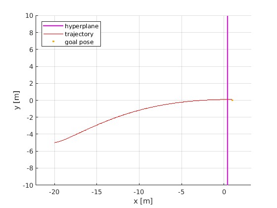
Hi, I have created a MPC for the trajectory generation of a vehicle in Matlab24a with acados. The interface i am using is the old one. I started simple by following the Race car example and it works fine without any additional constraint. But when i added an external constraint like a hyperplane for the collision avoidance, the acados is not been able to consider this constraint for the trajectory generation.
%% Solver parameters
compile_interface = ‘auto’;
nlp_solver = ‘sqp’;
qp_solver = ‘full_condensing_hpipm’;
nlp_solver_exact_hessian = ‘false’; % false=gauss_newton, true=exact
qp_solver_cond_N = 50; % for partial condensing
regularize_method = ‘no_regularize’;
sim_method = ‘erk’; % erk, irk, irk_gnsf
%% horizon parameters
N = 50;
T = 0.05; % time horizon length% Goal pose
xg = [1;0;deg2rad(0)];
%% model dynamics
[model, constraint] = MPC_KEM(param);
nx = length(model.x);
nu = length(model.u);
%% model to create the solver
ocp_model = acados_ocp_model();
%% acados ocp solver
ocp_model.set(‘name’, model.name);
ocp_model.set(‘T’, T);
% symbolics
ocp_model.set(‘sym_x’, model.x);
ocp_model.set(‘sym_u’, model.u);
ocp_model.set(‘sym_xdot’, model.xdot);
% dynamics
if (strcmp(sim_method, ‘erk’))
ocp_model.set(‘dyn_type’, ‘explicit’);
ocp_model.set(‘dyn_expr_f’, model.f_expl_expr);
else % irk irk_gnsf
ocp_model.set(‘dyn_type’, ‘implicit’);
ocp_model.set(‘dyn_expr_f’, model.f_impl_expr);
end% set initial condition
ocp_model.set(‘constr_x0’, model.x0);nbu = 2;
Jbu = zeros(nbu,nu);
Jbu(1,1) = 1;
Jbu(2,2) = 1;
ocp_model.set(‘constr_Jbu’, Jbu);
ocp_model.set(‘constr_lbu’, [model.v_min, model.delta_min]);
ocp_model.set(‘constr_ubu’, [model.v_max, model.delta_max]);ocp_model.set(‘constr_type’,‘BGH’);
nh = 1;
%ocp_model.set(‘constr_dim_h’,1);
ocp_model.set(‘constr_expr_h’, constraint.expr);
ocp_model.set(‘constr_lh’, […
constraint.hyper_min,…
]);
ocp_model.set(‘constr_uh’,[…
constraint.hyper_max,…
]);
ocp_model.set(‘constr_expr_h_e’, constraint.expr);
ocp_model.set(‘constr_lh_e’, -inf);
ocp_model.set(‘constr_uh_e’, 0);% set terminal condition
% Jbx_e = eye(nx);
% ocp_model.set(‘constr_Jbx_e’, Jbx_e);
% ocp_model.set(‘constr_lbx_e’, xg);
% ocp_model.set(‘constr_ubx_e’, xg);% set cost
ocp_model.set(‘cost_type’, ‘linear_ls’);
ocp_model.set(‘cost_type_e’, ‘linear_ls’);ny = nx +nu;
ny_e = nx;Vx = zeros(ny, nx);
Vx_e =zeros(ny_e, nx);
Vu = zeros(ny, nu);Vx(1:nx,:)= eye(nx);
Vx_e(1:nx,:)= eye(nx);
Vu(nx+1:end,:)= eye(nu);
ocp_model.set(‘cost_Vx’, Vx);
ocp_model.set(‘cost_Vx_e’, Vx_e);
ocp_model.set(‘cost_Vu’, Vu);% Define cost on states and input
Q = diag([2, 6, 10]);
R = eye(nu);
R(1,1) = 0.1;
R(2,2) = 0.5;
Qe = diag([5, 5, 20]);unscale = N/T;
W = unscale * blkdiag(Q, R);
W_e = Qe/unscale;
ocp_model.set(‘cost_W’, W);
ocp_model.set(‘cost_W_e’, W_e);% set initial reference
y_ref = zeros(ny,1);
y_ref_e = zeros(ny_e,1);
ocp_model.set(‘cost_y_ref’,y_ref);
ocp_model.set(‘cost_y_ref_e’,y_ref_e);%% acados ocp set opts
ocp_opts = acados_ocp_opts();
%ocp_opts.set(‘compile_interface’, compile_interface);
ocp_opts.set(‘param_scheme_N’, N);
ocp_opts.set(‘nlp_solver’, nlp_solver);
ocp_opts.set(‘nlp_solver_exact_hessian’, nlp_solver_exact_hessian);
ocp_opts.set(‘sim_method’, sim_method);
ocp_opts.set(‘sim_method_num_stages’, 4);
ocp_opts.set(‘sim_method_num_steps’, 3);
ocp_opts.set(‘qp_solver’, qp_solver);
%ocp_opts.set(‘regularize_method’, regularize_method);
ocp_opts.set(‘qp_solver_cond_N’, qp_solver_cond_N);
ocp_opts.set(‘nlp_solver_tol_stat’, 1e-4);
ocp_opts.set(‘nlp_solver_tol_eq’, 1e-4);
ocp_opts.set(‘nlp_solver_tol_ineq’, 1e-4);
ocp_opts.set(‘nlp_solver_tol_comp’, 1e-4);
%% create ocp solver
ocp_solver = acados_ocp(ocp_model, ocp_opts);
%% Simulate
Tf = 20;
Nsim = round(Tf/T);% initialize data structs
simX = zeros(Nsim, nx);
simU = zeros(Nsim, nu);
tcomp_sum = 0;
tcomp_max = 0;% initial state constraint
ocp_solver.set(‘constr_x0’, model.x0);
ocp_solver.set(‘constr_lbx’, model.x0, 0);
ocp_solver.set(‘constr_ubx’, model.x0, 0);% warm start/ setting trajectory initialization
ocp_solver.set(‘init_x’, model.x0 * ones(1,N+1));
ocp_solver.set(‘init_u’, zeros(nu,N));
ocp_solver.set(‘init_pi’,zeros(nx,N));tolerance = 1e-2;
% simulate
for i = 1:500
for j = 0:(N-1)
yref = [xg;0;0];
ocp_solver.set(‘cost_y_ref’,yref,j);
end
yref_N = xg;
ocp_solver.set(‘cost_y_ref_e’, yref_N);ocp_solver.solve(); status = ocp_solver.get('status'); if status ~= 0 && status ~= 2 error(sprintf('acados returned status %d in closed loop iteration %d. Exiting', status,1)); end x0 = ocp_solver.get('x',0); u0 = ocp_solver.get('u',0); for j = 1:nx simX(i,j)= x0(j); end for j = 1:nu simU(i,j) = u0(j); end % cHeck convergence pos_error = norm([x0(1) - xg(1), x0(2)-xg(2)]); if pos_error < tolerance fprintf('Converged at ietration %d\n', i); fprintf('Position error: %.4f m', pos_error); break; end x0 = shift_state(x0, u0, param.T,param); %x0 = ocp_solver.get('x',1); ocp_solver.set('constr_x0',x0); ocp_solver.set('constr_lbx',x0, 0); ocp_solver.set('constr_ubx', x0, 0);end
%% Plots
x_error= yref(1)-simX(end,1);
y_error = yref(2)-simX(end,2);
angle1 = yref(3); angle2 = simX(end,3);
diff = angle1 - angle2;
diff = atan2(sin(diff), cos(diff));
angle = diff;
thete_error_wrapped = rad2deg(angle);
theta_error = rad2deg(yref(3)-simX(end,3));figure(1); clf; hold on; axis equal;
x_hyper = linspace(-20,0,500);
xx_hyper = ones(size(x_hyper))*param.hyperplane;
hp = rotate_points(xx_hyper, linspace(-10,10,500),param);
plot(hp(1,:), hp(2,:), ‘m-’, ‘LineWidth’,1.5);
plot(simX(:,1),simX(:,2),‘r’);
hold on;
plot(yref(1),yref(2),‘.’);
grid on;figure(2);
subplot(3,1,1);
plot(simU(:,1));
grid on;subplot(3,1,2);
plot(simU(:,2));
grid on;subplot(3,1,3);
plot(simX(:,3));
grid on;function [model, constraint] = MPC_KEM(param)
import casadi.*
model = struct();
%constraint = struct();model_name = ‘CoupleMPC’;
%% Vehicle Parameter
L = param.L;
lf = param.lf;
lr = param.lr;
cone_apex = param.cone_apex;
hyperplane = param.hyperplane;
orientation = param.orientation;%% Casadi Model
x_pos = MX.sym(‘x_pos’);
y_pos = MX.sym(‘y_pos’);
theta = MX.sym(‘theta’);
x = vertcat(x_pos, y_pos, theta);% Controls
v = MX.sym(‘v’);
delta = MX.sym(‘delta’);
u = vertcat(v,delta);% xdot
x_pos_dot = MX.sym(‘x_pos_dot’);
y_pos_dot = MX.sym(‘y_pos_dot’);
theta_dot = MX.sym(‘theta_dot’);
xdot = vertcat(x_pos_dot, y_pos_dot, theta_dot);% algebraic variables
z = ;% parameters
p = ;% Dynamics
slip = atan((lr/L) * tan(delta));
f_expl = [ v * cos(theta + slip); …
v * sin(theta + slip); …
(v / lr) * sin(slip)];% Bounds
model.v_min = -1;
model.v_max = 1;model.delta_min = -deg2rad(25);
model.delta_max = deg2rad(25);% Define initial condition
model.x0 = [-20;5; deg2rad(0)];% Constraints
d = [x_pos;y_pos] - cone_apex;
Rotation = [cos(-orientation), -sin(-orientation);
sin(-orientation), cos(-orientation)];
dr = Rotation*d;
Xr = dr(1);
Collison_Avoidance = Xr - hyperplane;% Constraints bounds
constraint.hyper_min = -inf;
constraint.hyper_max = 0;% Define constraints struct
constraint.hyper = Function(‘Collison_Avoidance’, {x}, {Collison_Avoidance});
constraint.expr = Collison_Avoidance;% Define model struct
model.f_impl_expr = f_expl - xdot;
model.f_expl_expr = f_expl;
model.x = x;
model.u = u;
model.xdot = xdot;
model.z = z;
model.p = p;
model.name = model_name;
end
Why the acados is not been able to consider the constr_expr_h for the trajectory generation. I appreciate any help. Thanks