NMPC only solves for one control input

earthlertkit · April 8, 2025, 5:19pm

Hi everyone!

I am using acados with python to solve an NMPC for a simple position tracking quadrotor. My states are x = [p, q, v, \omega] and my control inputs are u = [T_{total}, M_x, M_y, M_z]. My only constraint is a box constraint on the total thrust where T_{min} < T < T_{max}. My weights only penalize the position error for now since I want to make sure everything is working properly first before fine tuning anything.

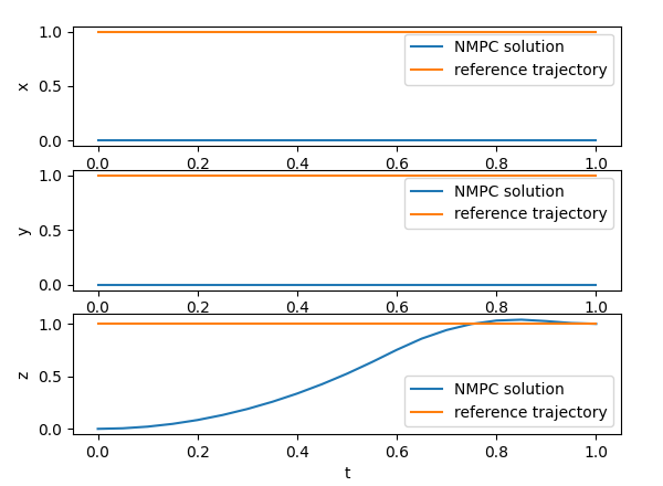
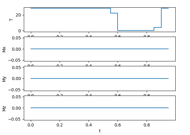
The issue is my solver seems to ONLY solve for the total thrust, and the other inputs are always zero and I can’t seem to figure out why. This causes my position tracking to not work in the x and y directions but work perfectly in the z direction. Below is a minimal example to replicate my issue.

import casadi as ca
import scipy.linalg
import matplotlib.pyplot as plt
from acados_template import AcadosModel, AcadosOcp, AcadosOcpSolver, AcadosSimSolver


def quat_multiply(q1, q2):

    w1 = q1[0]
    x1 = q1[1]
    y1 = q1[2]
    z1 = q1[3]

    w2 = q2[0]
    x2 = q2[1]
    y2 = q2[2]
    z2 = q2[3]

    w = w1*w2 - x1*x2 - y1*y2 - z1*z2
    x = w1*x2 + x1*w2 + y1*z2 - z1*y2
    y = w1*y2 - x1*z2 + y1*w2 + z1*x2
    z = w1*z2 + x1*y2 - y1*x2 + z1*w2

    return ca.vertcat(w, x, y, z)


###################################### Quadrotor parameters ##############################################

m = 2.02 # [kg]
Ix = 0.011 # [kg.m^2]
Iy = 0.015 # [kg.m^2]
Iz = 0.021 # [kg.m^2]
g = 9.81 # [m/s^2]
l = 0.26 # [m]
ct =  5.84e-6 # []
cq = 0.06*ct # []
T_min = 0 # [N]
T_hover = m*g # [N]
T_max = 28.3 # [N]

######################################### OCP settings ###################################################

# Discretization
dt = 0.05 # [s]
N_horizon = 20 # prediction horizon length

# NLP solver
nlp_solver = "SQP_RTI"

# QP solver
qp_solver = "PARTIAL_CONDENSING_HPIPM"
hessian_approx = "GAUSS_NEWTON"

# Integrator
integrator_type = "ERK"
sim_method_num_stages = 4
sim_method_num_steps = 1

# Cost function
cost_type = "LINEAR_LS" # Stage cost
cost_type_e = "LINEAR_LS" # Terminal cost

Q = np.diag([10, 10, 10,    # Position
             0, 0, 0, 0,    # Quaternions
             0, 0, 0,       # Velocity
             0, 0, 0,])     # Angular Velocity

QN = np.diag([10, 10, 10,   # Position
             0, 0, 0, 0,    # Quaternions
             0, 0, 0,       # Velocity
             0, 0, 0,])     # Angular Velocity

R = np.diag([0, 0, 0, 0])


################################## Symbolic state variables #####################

# Position
px = ca.SX.sym('px')
py = ca.SX.sym('py')
pz = ca.SX.sym('pz')

# Quaternions
q0 = ca.SX.sym('q0')
q1 = ca.SX.sym('q1')
q2 = ca.SX.sym('q2')
q3 = ca.SX.sym('q3')

# Velocity
vx = ca.SX.sym('vx')
vy = ca.SX.sym('vy')
vz = ca.SX.sym('vz')

# Angular velocity
wx = ca.SX.sym('wx')
wy = ca.SX.sym('wy')
wz = ca.SX.sym('wz')

### ############################ Symbolic control variables #####################

T = ca.SX.sym('T')
Mx = ca.SX.sym('Mx')
My = ca.SX.sym('My')
Mz = ca.SX.sym('Mz')

#################################### NMPC class ############################

class NMPC():

    def __init__(self):
        self.ocp = None
        self.solver = None
        self.simulator = None

        self.x0 = None
        self.u0 = None
        self.xN = None
        self.uN = None


    def model_setup(self):
        
        # Position dynamics
        pxDot = vx
        pyDot = vy
        pzDot = vz
 
        # Quaternion dynamics
        wq = ca.vertcat(0, wx, wy, wz)
        q = ca.vertcat(q0, q1, q2, q3)
        qDot = 0.5 * quat_multiply(q, wq)
        q0Dot = qDot[0]
        q1Dot = qDot[1]
        q2Dot = qDot[2]
        q3Dot = qDot[3]

        # Velocity dynamics
        Rq = ca.vertcat(ca.horzcat( 1 - 2*(q2**2 + q3**2),  2*(q1*q2 - q0*q3),      2*(q1*q3 + q0*q2)),
                        ca.horzcat( 2*(q1*q2 + q0*q3),      1 - 2*(q1**2 + q3**2),  2*(q2*q3 - q0*q1)),
                        ca.horzcat( 2*(q1*q3 - q0*q2),      2*(q2*q3 + q0*q1),      1 - 2*(q1**2 + q2**2)))
        F = ca.vertcat(0, 0, T)
        G = ca.vertcat(0, 0, g)
        vDot = 1/m * Rq @ F - G
        vxDot = vDot[0]
        vyDot = vDot[1]
        vzDot = vDot[2]

        # Angular velocity dynamics
        J = ca.diag([Ix, Iy, Iz])
        M = ca.vertcat(Mx, My, Mz)
        w = ca.vertcat(wx, wy, wz)
        wDot = ca.inv(J) @ (M - ca.cross(w, J @ w))
        wxDot = wDot[0]
        wyDot = wDot[1]
        wzDot = wDot[2]

        # States
        state = ca.vertcat(px, py, pz,
                           q0, q1, q2, q3,
                           vx, vy, vz,
                           wx, wy, wz)
        
        # Controls
        control = ca.vertcat(T, Mx, My, Mz)

        # Dynamics
        stateDot = ca.vertcat(pxDot, pyDot, pzDot,
                              q0Dot, q1Dot, q2Dot, q3Dot,
                              vxDot, vyDot, vzDot,
                              wxDot, wyDot, wzDot)

        return state, control, stateDot
    

    def ocp_setup(self, x0):

        ### Setting up model ###
        state, control, stateDot = self.model_setup()
        model = AcadosModel()
        model.name = "nmpc"

        model.x = state
        model.u = control
        model.f_expl_expr = stateDot

        ### Setting up acados solver ###
        ocp = AcadosOcp()
        ocp.model = model

        # Dimensions
        nx = state.size()[0]
        nu = control.size()[0]
        ny = nx + nu
        ny_e = nx

        # Control constraints
        ocp.constraints.idxbu = np.array([0])
        ocp.constraints.lbu = np.array([T_min])
        ocp.constraints.ubu = np.array([T_max])

        # Contuinity constraint
        self.x0 = x0
        ocp.constraints.x0 = self.x0

        # Cost function
        ocp.cost.cost_type = cost_type
        ocp.cost.cost_type_e = cost_type

        ocp.cost.W = scipy.linalg.block_diag(Q, R)
        ocp.cost.W_e = QN

        ocp.cost.Vx = np.vstack([
            np.eye(nx),
            np.zeros((nu, nx))
        ])
        ocp.cost.Vx_e = np.eye(nx)

        ocp.cost.Vu = np.vstack([
            np.zeros((nx, nu)),
            np.eye(nu)
        ])

        ocp.cost.yref = np.zeros((ny, 1))
        ocp.cost.yref_e = np.zeros((ny_e, 1))

        ### Acados solver settings ###
        ocp.solver_options.N_horizon = N_horizon
        ocp.solver_options.tf = N_horizon * dt
        ocp.solver_options.nlp_solver_type = nlp_solver
        ocp.solver_options.qp_solver = qp_solver
        ocp.solver_options.hessian_approx = hessian_approx
        ocp.solver_options.integrator_type = integrator_type
        ocp.solver_options.sim_method_num_stages = sim_method_num_stages
        ocp.solver_options.sim_method_num_steps = sim_method_num_steps

        ### Creating solver ###
        self.ocp = ocp
        self.solver = AcadosOcpSolver(ocp, json_file = "nmpc.json")
        self.integrator = AcadosSimSolver(ocp)


    def solve_ocp(self):
        
        # Solve ocp with multiple shooting and simulate with RK4
        self.u0 = self.solver.solve_for_x0(self.x0)

        # Retrieve solutions for all time steps
        nx = self.ocp.dims.nx
        nu = self.ocp.dims.nu
        self.xN = np.zeros((nx, N_horizon+1))
        self.uN = np.zeros((nu, N_horizon))

        for i in range(N_horizon):
            self.xN[:, i] = np.reshape(self.solver.get(i, 'x'), (nx,))
            self.uN[:, i] = np.reshape(self.solver.get(i, 'u'), (nu,))

        self.xN[:, N_horizon] = np.reshape(self.solver.get(N_horizon, 'x'), (nx,))

        return self.x0, self.u0, self.xN, self.uN
    

if __name__ == "__main__":
    controller = NMPC()

    x0 = np.array([0, 0, 0, 1, 0, 0, 0, 0, 0, 0, 0, 0, 0])
    controller.ocp_setup(x0)

    yref_array = np.zeros((17, N_horizon+1)) 
    yref = np.array([1, 1, 1, 1, 0, 0, 0, 0, 0, 0, 0, 0, 0, 0, 0, 0, 0])
    for i in range(N_horizon):
        controller.solver.cost_set(i, "yref", yref)
        yref_array[:, i] = controller.solver.cost_get(i, "yref")
    controller.solver.cost_set(N_horizon, "yref", yref[:13])
    yref_array[:13, -1] = controller.solver.cost_get(N_horizon, "yref")

    # NMPC solver (current pos = [0, 0, 0], target_pos = [1, 1, 1])
    x0, u0, xN, uN = controller.solve_ocp()

    # Position plot
    t = np.linspace(0, N_horizon * dt, N_horizon + 1)

    fig, ax = plt.subplots(3, 1)

    ax[0].plot(t, xN[0, :], label='NMPC solution')
    ax[0].plot(t, yref_array[0, :], label='reference trajectory')
    ax[0].set_ylabel('x')
    ax[0].set_xlabel('t')
    ax[0].legend()

    ax[1].plot(t, xN[1, :], label='NMPC solution')
    ax[1].plot(t, yref_array[1, :], label='reference trajectory')
    ax[1].set_ylabel('y')
    ax[1].set_xlabel('t')
    ax[1].legend()

    ax[2].plot(t, xN[2, :], label='NMPC solution')
    ax[2].plot(t, yref_array[2, :], label='reference trajectory')
    ax[2].set_ylabel('z')
    ax[2].set_xlabel('t')
    ax[2].legend()

    # Control plot
    fig, ax = plt.subplots(4, 1)

    ax[0].plot(t[:-1], uN[0, :], drawstyle='steps-post')
    ax[0].set_ylabel('T')
    ax[0].set_xlabel('t')
    
    ax[1].plot(t[:-1], uN[1, :], drawstyle='steps-post')
    ax[1].set_ylabel('Mx')
    ax[1].set_xlabel('t')
    
    ax[2].plot(t[:-1], uN[2, :], drawstyle='steps-post')
    ax[2].set_ylabel('My')
    ax[2].set_xlabel('t')
    
    ax[3].plot(t[:-1], uN[3, :], drawstyle='steps-post')
    ax[3].set_ylabel('Mz')
    ax[3].set_xlabel('t')

    plt.show()

This is what my graphs are from running the code:

Any help would be greatly appreciated!

kaethe · April 8, 2025, 5:38pm

Hi
could you check whether the solve ist successful, i.e. do you get status 0?
What is the output of print_statistics?

earthlertkit · April 8, 2025, 5:47pm

Thank you for your swift reply!

I ran print(controller.solver.get_status())) and the output is 0.
I ran print(controller.solver.print_statistics())) and the output is:

Does this mean the solve is successful?

kaethe · April 8, 2025, 6:56pm

Could you change nlp_solver = "SQP_RTI" to nlp_solver = "SQP" and again check the status and the statistics? At the moment you solve only a single QP.

In general, I would also recommend to add some weight on all controls (can be very small) in order for the reduced Hessian to be positive definite.

earthlertkit · April 8, 2025, 7:23pm

I changed all the weights that are 0 to 1e-6 instead, and I changed the solver to SQP as you suggested. However, this time the output is:

with the error:

raise Exception(f'acados acados_ocp_solver returned status {status}')
Exception: acados acados_ocp_solver returned status 4

kaethe · April 8, 2025, 7:48pm

Ok, so this means that your problem could not be solved and the problem seems to be the dynamics as the equality residual ist not converging.

Did you try to simulate the system dynamics outside of an OCP formulation using an AcadosSimSolver? Could you come up with a better initial guess? E.g. a hovering position and the corresponding controls?

earthlertkit · April 10, 2025, 3:37am

I tested the dynamics with the AcadosSimSolver and verified that it was correct. I played around with the constraints, weight, and target waypoint a bit more and finally found a configuration where it works! The only thing I’m worried about is that this only works using SQP, and when I try to use SQP_RTI it breaks again. Not sure how I would fix this

kaethe · April 10, 2025, 7:08am

This is expected behaviour as RTI is meant for fast closed-loop control. With RTI, the OCP is not solved (only a single QP approximation of the nonlinear OCP is). If you start from a good initial guess and apply the solution in an NMPC fashion, you can typically expect good closed-loop performance.

Compare also the references here:

earthlertkit · April 14, 2025, 6:03am

I see! Is there a way to come up with a good initial guess or is it just trial and error? Also, would I need to come up with another initial guess again when I want to solve the OCP at the next time step?

Also, this is unrelated but what does the variable res_stat mean? Why does it increase in the first iteration before decreasing?

kaethe · April 14, 2025, 6:22am

You only need an initial guess for the very first OCP, afterwards acados will use the previous solution as initial guess for the next OCP.

Finding a good initial guess is typically done heuristically. For a quadrotor you could use a hovering state and corresponding controls.

The stationarity residual is the gradient of the Lagrange function. There is typically no guarantee that it will decrease monotonically (In the first iteration stationarity increases, but on the other hand infeasibility of the equality constraints decreases)