Hi ![]()
I am new to ACADOS and MPC in general.
I am trying to implement Acados numerical solver for finding the solution of the MPC problem for trajectory optimization of a Mobile robot
I am using Python interface and I want to implement two different cost functions:
- The cost function of minimizing the error between real and initial trajectory has the following general formula
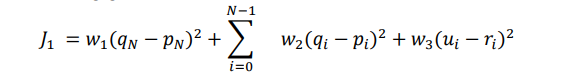
where
- q and u are the output and input vectors of the trajectory of the robot
- p and r are the output and input vector of the trajectory,
- w_1 , w_2 , w_3 are weights.
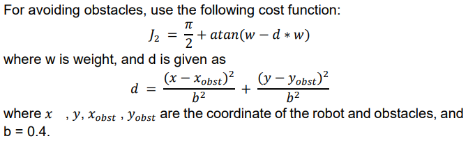
- Control inputs are r = [a, w]^T=0
- Cost function for avoiding obstacles:
I was told to use NONLINEAR_LS for defining the cost functions. but I am not sure how to combine two different costs.
My code:
Model
def mobile_robot_model():


    model_name = 'mobile_robot'

    # Define symbolic variables (states)
    x = ca.MX.sym('x')
    y = ca.MX.sym('y')
    v = ca.MX.sym('v')
    theta = ca.MX.sym('theta')

    # Control
    a = ca.MX.sym('a')  # acceleration
    w = ca.MX.sym('w')  # angular velocity

    # Define state and control vectors
    states = ca.vertcat(x, y, v, theta)
    controls = ca.vertcat(a, w)
    rhs = [v*ca.cos(theta), v*ca.sin(theta), a, w]
    x_dot = ca.MX.sym('x_dot', len(rhs))

    # Create a CasADi function for the continuous-time dynamics
    continuous_dynamics = ca.Function(
        'continuous_dynamics',
        [states, controls],
        [ca.vcat(rhs)],
        ["state", "control_input"],
        ["rhs"]
    )

    f_impl = x_dot - continuous_dynamics(states, controls)

    model = AcadosModel()

    model.f_expl_expr = continuous_dynamics(states, controls)
    model.f_impl_expr = f_impl
    model.x = states
    model.xdot = x_dot
    model.u = controls
    model.p = []
    model.name = model_name

    return model
Solver:
def create_ocp_solver():

    # Create AcadosOcp object
    ocp = AcadosOcp()

    # Set up the optimization problem
    model = mobile_robot_model()
    ocp.model = model

    # --------------------PARAMETERS--------------
    # constants
    nx = model.x.size()[0]
    nu = model.u.size()[0]
    T = 30
    N = 100
    n_params = len(model.p)

    # Setting initial conditions
    ocp.dims.N = N
    ocp.dims.nx = nx
    ocp.dims.nu = nu
    ocp.solver_options.tf = T

    # initial state
    x_ref = np.zeros(nx)

    # Set initial condition for the robot
    ocp.constraints.x0 = x_ref

    # initialize parameters
    ocp.dims.np = n_params
    ocp.parameter_values = np.zeros(n_params)

    # ---------------------CONSTRAINTS------------------
    # Define constraints on states and control inputs
    ocp.constraints.lbu = np.array([-0.1, -0.3])  # Lower bounds on control inputs
    ocp.constraints.ubu = np.array([0.1, 0.3])    # Upper bounds on control inputs
    ocp.constraints.lu = np.array([100, 100, 1, 10])  # Upper bounds on states
    ocp.constraints.idxbu = np.array([0, 1])  # for indices 0 & 1

    # ---------------------COSTS--------------------------

    # Define J1 and J2
    # Define cost_y_expr, cost_y_expr_e
    # Define W and W_e
    # Define yref and yref_e

    ocp.cost.cost_type = 'NONLINEAR_LS'
    ocp.cost.cost_type_e = 'NONLINEAR_LS'

    X = ocp.model.x
    U = ocp.model.u

    # Cost weights
    w1 = 1.0  # adjust as needed
    w2 = 1.0  # adjust as needed
    w3 = 1.0  # adjust as needed
    w = 1.0

    J2 = obstacle_cost(X, w)

    # Parameters:
    ocp.model.cost_y_expr = J2
    ocp.model.cost_y_expr_e = J2

    ocp.cost.W = np.eye(1)
    ocp.cost.W_e = np.eye(1)

    ocp.cost.yref = np.array([0])
    ocp.cost.yref_e = np.array([0])

    # ---------------------SOLVER-------------------------
    ocp.solver_options.qp_solver = 'PARTIAL_CONDENSING_HPIPM'
    ocp.solver_options.hessian_approx = 'GAUSS_NEWTON'
    ocp.solver_options.integrator_type = 'ERK'
    ocp.solver_options.nlp_solver_type = 'SQP_RTI'

    # Set up Acados solver
    acados_solver = AcadosOcpSolver(ocp, json_file='acados_ocp.json')
    acados_integrator = AcadosSimSolver(ocp, json_file='acados_ocp.json')

    return ocp, acados_solver, acados_integrator
I have implemented the cost function for obstacles but not for the trajectory.
Thank you for the help ![]()