Hi everyone,
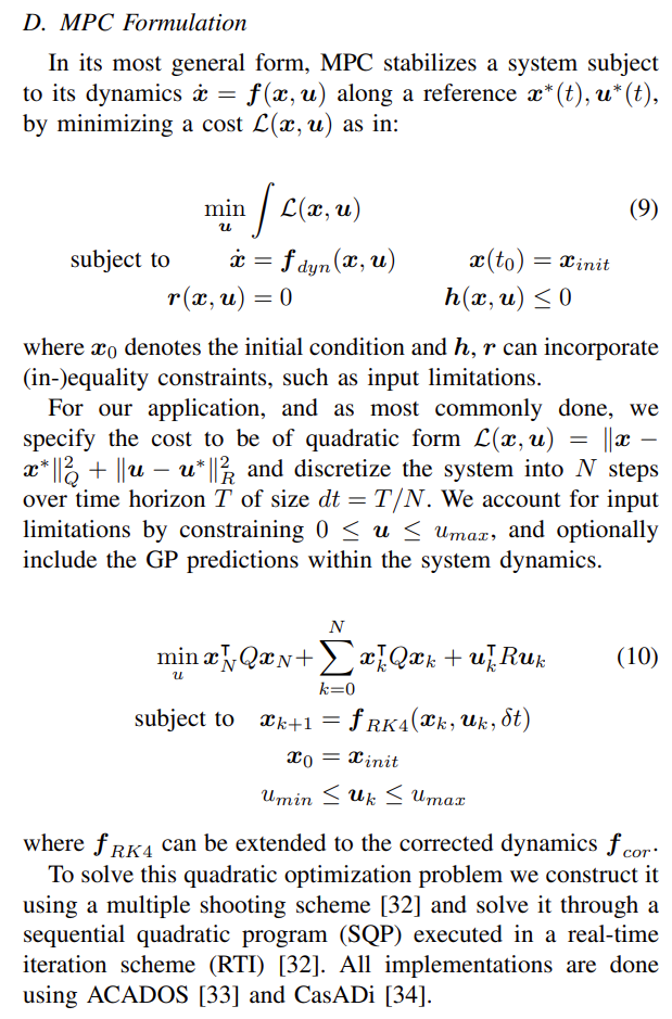
I am working on a simplified version of a UAV Model Predictive Control (MPC) problem and need assistance with adapting the code to solve a maximization problem. The original code is designed for minimization, but my goal is to modify it to handle a maximization problem instead.
Objective: I am trying to develop an MPC for a UAV that aims to maximize its distance from a moving point (set as the reference state). The objective is to maximize the position difference between the UAV and the moving point. The reference state input to this MPC is the instantaneous state of the moving point.
I have made some modifications to the original code to achieve this, but I encountered the following error:
QP solver returned error status 3 in SQP iteration 1, QP iteration 1.
From my research on the forum, this error suggests that the problem has become infeasible to solve. However, I am not sure why this is happening or how to resolve it. I am uncertain if the issue lies in the solver options or if simply negating the weighting matrix is causing infeasibility. In theory, negating the original objective function (which aims to minimize the distance to the moving point) should lead the UAV to maximize the distance instead.
import os
import sys
import shutil
import casadi as cs
import numpy as np
from copy import copy
from acados_template import AcadosOcp, AcadosOcpSolver, AcadosModel
from src.quad_mpc.quad_3d import Quadrotor3D
from src.model_fitting.gp import GPEnsemble
from src.utils.utils import skew_symmetric, v_dot_q, safe_mkdir_recursive, quaternion_inverse
from src.utils.quad_3d_opt_utils import discretize_dynamics_and_cost


class Quad3DOptimizer:
    def __init__(self, quad, t_horizon=1, n_nodes=20,
                 q_cost=None, r_cost=None, q_mask=None,
                 B_x=None, gp_regressors=None, rdrv_d_mat=None,
                 model_name="quad_3d_acados_mpc", solver_options=None, maximize=False):
        """
        :param quad: quadrotor object
        :type quad: Quadrotor3D
        :param t_horizon: time horizon for MPC optimization
        :param n_nodes: number of optimization nodes until time horizon
        :param q_cost: diagonal of Q matrix for LQR cost of MPC cost function. Must be a numpy array of length 12.
        :param r_cost: diagonal of R matrix for LQR cost of MPC cost function. Must be a numpy array of length 4.
        :param B_x: dictionary of matrices that maps the outputs of the gp regressors to the state space.
        :param gp_regressors: Gaussian Process ensemble for correcting the nominal model
        :type gp_regressors: GPEnsemble
        :param q_mask: Optional boolean mask that determines which variables from the state compute towards the cost
        function. In case no argument is passed, all variables are weighted.
        :param solver_options: Optional set of extra options dictionary for solvers.
        :param rdrv_d_mat: 3x3 matrix that corrects the drag with a linear model according to Faessler et al. 2018. None
        if not used
        """

        # Weighted squared error loss function q = (p_xyz, a_xyz, v_xyz, r_xyz), r = (u1, u2, u3, u4)
        if maximize:
            q_cost = np.array([-0.5, -0.5, -0.5, 0.1, 0.1, 0.1, 0.05, 0.05, 0.05, 0.01, 0.01, 0.01])
            r_cost = np.array([1.0, 1.0, 1.0, 1.0])

            q_mask = np.array([1, 1, 1, 1, 1, 1, 1, 1, 1, 1, 1, 1]).T
        else:
            q_cost = np.array([0.5, 0.5, 0.5, 0.1, 0.1, 0.1, 0.05, 0.05, 0.05, 0.01, 0.01, 0.01])
            r_cost = np.array([1.0, 1.0, 1.0, 1.0])

            q_mask = np.array([1, 1, 1, 1, 1, 1, 1, 1, 1, 1, 1, 1]).T

        self.maximize =  maximize

        self.T = t_horizon  # Time horizon
        self.N = n_nodes  # number of control nodes within horizon

        self.quad = quad

        self.max_u = quad.max_input_value
        self.min_u = quad.min_input_value
        # print(quad.max_input_value)
        # print(quad.min_input_value)

        # Declare model variables
        self.p = cs.MX.sym('p', 3)  # position
        self.q = cs.MX.sym('a', 4)  # angle quaternion (wxyz)
        self.v = cs.MX.sym('v', 3)  # velocity
        self.r = cs.MX.sym('r', 3)  # angle rate

        # Full state vector (13-dimensional)
        self.x = cs.vertcat(self.p, self.q, self.v, self.r)
        self.state_dim = 13

        # Control input vector
        u1 = cs.MX.sym('u1')
        u2 = cs.MX.sym('u2')
        u3 = cs.MX.sym('u3')
        u4 = cs.MX.sym('u4')
        self.u = cs.vertcat(u1, u2, u3, u4)

        # Nominal model equations symbolic function (no GP)
        self.quad_xdot_nominal = self.quad_dynamics(rdrv_d_mat)

        # Linearized model dynamics symbolic function
        self.quad_xdot_jac = self.linearized_quad_dynamics()

        # Initialize objective function, 0 target state and integration equations
        self.L = None
        self.target = None

        self.gp_reg_ensemble = None

        # Declare model variables for GP prediction (only used in real quadrotor flight with EKF estimator).
        # Will be used as initial state for GP prediction as Acados parameters.
        self.gp_p = cs.MX.sym('gp_p', 3)
        self.gp_q = cs.MX.sym('gp_a', 4)
        self.gp_v = cs.MX.sym('gp_v', 3)
        self.gp_r = cs.MX.sym('gp_r', 3)
        self.gp_x = cs.vertcat(self.gp_p, self.gp_q, self.gp_v, self.gp_r)

        # The trigger variable is used to tell ACADOS to use the additional GP state estimate in the first optimization
        # node and the regular integrated state in the rest
        self.trigger_var = cs.MX.sym('trigger', 1)

        # Build full model. Will have 13 variables. self.dyn_x contains the symbolic variable that
        # should be used to evaluate the dynamics function. It corresponds to self.x if there are no GP's, or
        # self.x_with_gp otherwise
        acados_models, nominal_with_gp = self.acados_setup_model(
            self.quad_xdot_nominal(x=self.x, u=self.u)['x_dot'], model_name)

        # Convert dynamics variables to functions of the state and input vectors
        self.quad_xdot = {}
        for dyn_model_idx in nominal_with_gp.keys():
            dyn = nominal_with_gp[dyn_model_idx]
            self.quad_xdot[dyn_model_idx] = cs.Function('x_dot', [self.x, self.u], [dyn], ['x', 'u'], ['x_dot'])

        # ### Setup and compile Acados OCP solvers ### #
        self.acados_ocp_solver = {}

        # Add one more weight to the rotation (use quaternion norm weighting in acados)
        q_diagonal = np.concatenate((q_cost[:3], np.mean(q_cost[3:6])[np.newaxis], q_cost[3:]))

        # Ensure current working directory is current folder
        os.chdir(os.path.dirname(os.path.realpath(__file__)))
        self.acados_models_dir = '../../acados_models'
        safe_mkdir_recursive(os.path.join(os.getcwd(), self.acados_models_dir))

        for key, key_model in zip(acados_models.keys(), acados_models.values()):
            nx = key_model.x.size()[0]
            nu = key_model.u.size()[0]
            ny = nx + nu
            n_param = key_model.p.size()[0] if isinstance(key_model.p, cs.MX) else 0

            acados_source_path = os.environ['ACADOS_SOURCE_DIR']
            sys.path.insert(0, '../common')

            # Create OCP object to formulate the optimization
            ocp = AcadosOcp()
            ocp.acados_include_path = acados_source_path + '/include'
            ocp.acados_lib_path = acados_source_path + '/lib'
            ocp.model = key_model
            ocp.dims.N = self.N
            ocp.solver_options.tf = t_horizon

            # Initialize parameters
            ocp.dims.np = n_param
            ocp.parameter_values = np.zeros(n_param)

            ocp.cost.cost_type = 'LINEAR_LS'
            ocp.cost.cost_type_e = 'LINEAR_LS'


            ocp.cost.W = np.diag(np.concatenate((q_diagonal, r_cost)))
            ocp.cost.W_e = np.diag(q_diagonal)
            print("min")
            terminal_cost = 0 if solver_options is None or not solver_options["terminal_cost"] else 1
            ocp.cost.W_e *= terminal_cost

            ocp.cost.Vx = np.zeros((ny, nx))
            ocp.cost.Vx[:nx, :nx] = np.eye(nx)
            ocp.cost.Vu = np.zeros((ny, nu))
            ocp.cost.Vu[-4:, -4:] = np.eye(nu)

            ocp.cost.Vx_e = np.eye(nx)

            # Initial reference trajectory (will be overwritten)
            x_ref = np.zeros(nx)
            ocp.cost.yref = np.concatenate((x_ref, np.array([0.0, 0.0, 0.0, 0.0])))
            ocp.cost.yref_e = x_ref

            # Initial state (will be overwritten)
            ocp.constraints.x0 = x_ref

            # Set constraints
            ocp.constraints.lbu = np.array([self.min_u] * 4)
            ocp.constraints.ubu = np.array([self.max_u] * 4)
            ocp.constraints.idxbu = np.array([0, 1, 2, 3])

            # Solver options
            ocp.solver_options.qp_solver = 'FULL_CONDENSING_HPIPM'
            ocp.solver_options.hessian_approx = 'GAUSS_NEWTON'
            ocp.solver_options.integrator_type = 'ERK'
            ocp.solver_options.print_level = 0

            ocp.solver_options.nlp_solver_type = 'SQP_RTI' if solver_options is None else solver_options["solver_type"]

            # Compile acados OCP solver if necessary
            json_file = os.path.join(self.acados_models_dir, key_model.name + '_acados_ocp.json')
            self.acados_ocp_solver[key] = AcadosOcpSolver(ocp, json_file=json_file)


    def acados_setup_model(self, nominal, model_name):
        """
        Builds an Acados symbolic models using CasADi expressions.
        :param model_name: name for the acados model. Must be different from previously used names or there may be
        problems loading the right model.
        :param nominal: CasADi symbolic nominal model of the quadrotor: f(self.x, self.u) = x_dot, dimensions 13x1.
        :return: Returns a total of three outputs, where m is the number of GP's in the GP ensemble, or 1 if no GP:
            - A dictionary of m AcadosModel of the GP-augmented quadrotor
            - A dictionary of m CasADi symbolic nominal dynamics equations with GP mean value augmentations (if with GP)
        :rtype: dict, dict, cs.MX
        """

        def fill_in_acados_model(x, u, p, dynamics, name):

            x_dot = cs.MX.sym('x_dot', dynamics.shape)
            f_impl = x_dot - dynamics

            # Dynamics model
            model = AcadosModel()
            model.f_expl_expr = dynamics
            model.f_impl_expr = f_impl
            model.x = x
            model.xdot = x_dot
            model.u = u
            model.p = p
            model.name = name

            return model

        acados_models = {}
        dynamics_equations = {}

        # No available GP so return nominal dynamics
        dynamics_equations[0] = nominal

        x_ = self.x
        dynamics_ = nominal

        acados_models[0] = fill_in_acados_model(x=x_, u=self.u, p=[], dynamics=dynamics_, name=model_name)

        return acados_models, dynamics_equations

    def quad_dynamics(self):
        """
        Symbolic dynamics of the 3D quadrotor model. The state consists on: [p_xyz, a_wxyz, v_xyz, r_xyz]^T, where p
        stands for position, a for angle (in quaternion form), v for velocity and r for body rate. The input of the
        system is: [u_1, u_2, u_3, u_4], i.e. the activation of the four thrusters.

        :param rdrv_d: a 3x3 diagonal matrix containing the D matrix coefficients for a linear drag model as proposed
        by Faessler et al.

        :return: CasADi function that computes the analytical differential state dynamics of the quadrotor model.
        Inputs: 'x' state of quadrotor (6x1) and 'u' control input (2x1). Output: differential state vector 'x_dot'
        (6x1)
        """

        x_dot = cs.vertcat(self.p_dynamics(), self.q_dynamics(), self.v_dynamics(), self.w_dynamics())
        return cs.Function('x_dot', [self.x[:13], self.u], [x_dot], ['x', 'u'], ['x_dot'])

    def p_dynamics(self):
        return self.v

    def q_dynamics(self):
        return 1 / 2 * cs.mtimes(skew_symmetric(self.r), self.q)

    def v_dynamics(self):
        """
        :param rdrv_d: a 3x3 diagonal matrix containing the D matrix coefficients for a linear drag model as proposed
        by Faessler et al. None, if no linear compensation is to be used.
        """

        f_thrust = self.u * self.quad.max_thrust
        g = cs.vertcat(0.0, 0.0, 9.81)
        a_thrust = cs.vertcat(0.0, 0.0, f_thrust[0] + f_thrust[1] + f_thrust[2] + f_thrust[3]) / self.quad.mass

        v_dynamics = v_dot_q(a_thrust, self.q) - g

        return v_dynamics

    def w_dynamics(self):
        f_thrust = self.u * self.quad.max_thrust

        y_f = cs.MX(self.quad.y_f)
        x_f = cs.MX(self.quad.x_f)
        c_f = cs.MX(self.quad.z_l_tau)
        return cs.vertcat(
            (cs.mtimes(f_thrust.T, y_f) + (self.quad.J[1] - self.quad.J[2]) * self.r[1] * self.r[2]) / self.quad.J[0],
            (-cs.mtimes(f_thrust.T, x_f) + (self.quad.J[2] - self.quad.J[0]) * self.r[2] * self.r[0]) / self.quad.J[1],
            (cs.mtimes(f_thrust.T, c_f) + (self.quad.J[0] - self.quad.J[1]) * self.r[0] * self.r[1]) / self.quad.J[2])

    def linearized_quad_dynamics(self):
        """
        Jacobian J matrix of the linearized dynamics specified in the function quad_dynamics. J[i, j] corresponds to
        the partial derivative of f_i(x) wrt x(j).

        :return: a CasADi symbolic function that calculates the 13 x 13 Jacobian matrix of the linearized simplified
        quadrotor dynamics
        """

        jac = cs.MX(self.state_dim, self.state_dim)

        # Position derivatives
        jac[0:3, 7:10] = cs.diag(cs.MX.ones(3))

        # Angle derivatives
        jac[3:7, 3:7] = skew_symmetric(self.r) / 2
        jac[3, 10:] = 1 / 2 * cs.horzcat(-self.q[1], -self.q[2], -self.q[3])
        jac[4, 10:] = 1 / 2 * cs.horzcat(self.q[0], -self.q[3], self.q[2])
        jac[5, 10:] = 1 / 2 * cs.horzcat(self.q[3], self.q[0], -self.q[1])
        jac[6, 10:] = 1 / 2 * cs.horzcat(-self.q[2], self.q[1], self.q[0])

        # Velocity derivatives
        a_u = (self.u[0] + self.u[1] + self.u[2] + self.u[3]) * self.quad.max_thrust / self.quad.mass
        jac[7, 3:7] = 2 * cs.horzcat(a_u * self.q[2], a_u * self.q[3], a_u * self.q[0], a_u * self.q[1])
        jac[8, 3:7] = 2 * cs.horzcat(-a_u * self.q[1], -a_u * self.q[0], a_u * self.q[3], a_u * self.q[2])
        jac[9, 3:7] = 2 * cs.horzcat(0, -2 * a_u * self.q[1], -2 * a_u * self.q[1], 0)

        # Rate derivatives
        jac[10, 10:] = (self.quad.J[1] - self.quad.J[2]) / self.quad.J[0] * cs.horzcat(0, self.r[2], self.r[1])
        jac[11, 10:] = (self.quad.J[2] - self.quad.J[0]) / self.quad.J[1] * cs.horzcat(self.r[2], 0, self.r[0])
        jac[12, 10:] = (self.quad.J[0] - self.quad.J[1]) / self.quad.J[2] * cs.horzcat(self.r[1], self.r[0], 0)

        return cs.Function('J', [self.x, self.u], [jac])

    def set_reference_state(self, x_target=None, u_target=None):
        """
        Sets the target state and pre-computes the integration dynamics with cost equations
        :param x_target: 13-dimensional target state (p_xyz, a_wxyz, v_xyz, r_xyz)
        :param u_target: 4-dimensional target control input vector (u_1, u_2, u_3, u_4)
        """

        if x_target is None:
            print("x_target is None")
            x_target = [[0, 0, 0], [1, 0, 0, 0], [0, 0, 0], [0, 0, 0]]
        if u_target is None:
            print("u_target is None")
            u_target = [0, 0, 0, 0]

        # Set new target state
        self.target = copy(x_target)

        ref = np.concatenate([x_target[i] for i in range(4)])
        #  Transform velocity to body frame
        v_b = v_dot_q(ref[7:10], quaternion_inverse(ref[3:7]))
        ref = np.concatenate((ref[:7], v_b, ref[10:]))

        # Determine which dynamics model to use based on the GP optimal input feature region. Should get one for each
        # output dimension of the GP
        gp_ind = 0

        ref = np.concatenate((ref, u_target))

        for j in range(self.N):
            self.acados_ocp_solver[gp_ind].set(j, "yref", ref)
        self.acados_ocp_solver[gp_ind].set(self.N, "yref", ref[:-4])

        return gp_ind

    def discretize_f_and_q(self, t_horizon, n, m=1, i=0, use_gp=True, use_model=0):
        """
        Discretize the model dynamics and the pre-computed cost function if available.
        :param t_horizon: time horizon in seconds
        :param n: number of control steps until time horizon
        :param m: number of integration steps per control step
        :param i: Only used for trajectory tracking. Index of cost function to use.
        :param use_gp: Whether to use the dynamics with the GP correction or not.
        :param use_model: integer, select which model to use from the available options.
        :return: the symbolic, discretized dynamics. The inputs of the symbolic function are x0 (the initial state) and
        p, the control input vector. The outputs are xf (the updated state) and qf. qf is the corresponding cost
        function of the integration, which is calculated from the pre-computed discrete-time model dynamics (self.L)
        """

        dynamics = self.quad_xdot[use_model] if use_gp else self.quad_xdot_nominal

        # Call with self.x_with_gp even if use_gp=False
        return discretize_dynamics_and_cost(t_horizon, n, m, self.x, self.u, dynamics, self.L, i)

    def run_optimization(self, initial_state=None, use_model=0, return_x=False):
        """
        Optimizes a trajectory to reach the pre-set target state, starting from the input initial state, that minimizes
        the quadratic cost function and respects the constraints of the system

        :param initial_state: 13-element list of the initial state. If None, 0 state will be used
        :param use_model: integer, select which model to use from the available options.
        :param return_x: bool, whether to also return the optimized sequence of states alongside with the controls.
        :param gp_regression_state: 13-element list of state for GP prediction. If None, initial_state will be used.
        :return: optimized control input sequence (flattened)
        """

        if initial_state is None:
            print("initial_state is None")
            initial_state = [0, 0, 0] + [1, 0, 0, 0] + [0, 0, 0] + [0, 0, 0]

        # Set initial state. Add gp state if needed
        x_init = initial_state
        x_init = np.stack(x_init)

        # Set initial condition, equality constraint
        self.acados_ocp_solver[use_model].set(0, 'lbx', x_init)
        self.acados_ocp_solver[use_model].set(0, 'ubx', x_init)

        # Solve OCP
        print("ready to solve the op")
        self.acados_ocp_solver[use_model].solve()

        # Get u
        w_opt_acados = np.ndarray((self.N, 4))
        x_opt_acados = np.ndarray((self.N + 1, len(x_init)))
        x_opt_acados[0, :] = self.acados_ocp_solver[use_model].get(0, "x")
        for i in range(self.N):
            w_opt_acados[i, :] = self.acados_ocp_solver[use_model].get(i, "u")
            x_opt_acados[i + 1, :] = self.acados_ocp_solver[use_model].get(i + 1, "x")

        w_opt_acados = np.reshape(w_opt_acados, (-1))
        return w_opt_acados if not return_x else (w_opt_acados, x_opt_acados)
The Debugging the solver’s output just generated something like
Thanks for your help