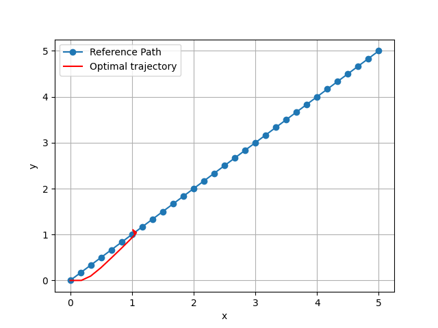
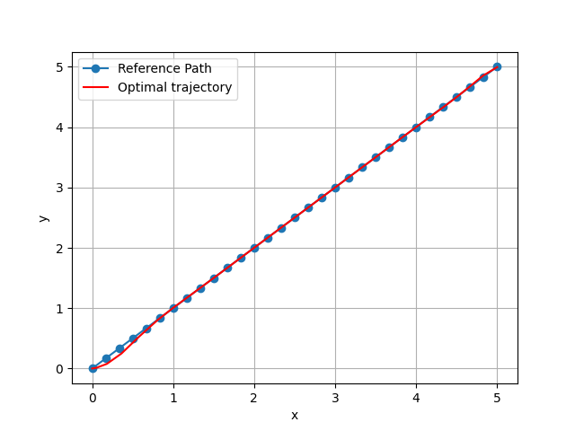
Hi ![]()
I am trying to write an acados numerical solver for Kinematic Model of a mobile robot in Python.
The task is pretty straight forward, I have 4 state variables [x,y,v,theta] and 2 control variables [a,w] (acceleration and angular velocity) and the robot needs start at (0,0) and finish at (5,5), initial and final velocity and orientation angle should be 0.
Solver:
def desired_trajectory(N):
    # Define parameters
    initial_position = (0, 0)
    final_position = (5, 5)

    # Linear interpolation for positions
    x = np.linspace(initial_position[0], final_position[0], N+1)
    y = np.linspace(initial_position[1], final_position[1], N+1)

    print(x[N], y[N])

    # Calculate v and theta for each pair of x and y
    v = 0.3 * np.ones(31)
    theta = np.arctan2(y, x)
    v[0] = 0
    v[N] = 0
    theta[N] = 0

    # Combine into p
    p = np.vstack((x, y, v, theta)).T

    a = np.zeros(len(x))  # Acceleration
    w = np.zeros(len(x))  # Angular velocity

    # Combine control variables into matrix r
    r = np.vstack((a, w)).T

    return p, r


def create_ocp_solver():
    """
    Create Acados solver for trajectory optimization.
    """

    # Create AcadosOcp object
    ocp = AcadosOcp()

    # Set up the optimization problem
    model = mobile_robot_model()
    ocp.model = model

    # --------------------PARAMETERS--------------
    # constants
    nx = model.x.size()[0]
    nu = model.u.size()[0]
    N = 30  # Prediction horizon (works for N =200)

    # Setting initial conditions
    ocp.dims.N = N
    ocp.dims.nx = nx
    ocp.dims.nu = nu

    # Set initial condition for the robot
    ocp.constraints.x0 = np.array([0, 0, 0, 0])

    # ---------------------CONSTRAINTS------------------
    # Define constraints on states and control inputs
    ocp.constraints.idxbu = np.array([0, 1])  # indices 0 & 1 of u
    ocp.constraints.idxbx = np.array([0, 1, 2, 3])  # indices 0...3 of x
    ocp.constraints.lbu = np.array([-0.1, -0.3])  # Lower bounds on control inputs
    ocp.constraints.ubu = np.array([0.1, 0.3])  # Upper bounds on control inputs
    ocp.constraints.lbx = np.array([-100, -100, 0, -10])  # Lower bounds on states
    ocp.constraints.ubx = np.array([100, 100, 1, 10])  # Upper bounds on states
    # ---------------------COSTS--------------------------
    # Set up the cost function
    ocp.cost.cost_type = "NONLINEAR_LS"
    ocp.cost.cost_type_e = "NONLINEAR_LS"

    X = ocp.model.x
    U = ocp.model.u

    ocp.model.cost_y_expr = ca.vertcat(X, U)
    ocp.model.cost_y_expr_e = X

    ocp.cost.yref = np.zeros(nx + nu)
    ocp.cost.yref_e = np.zeros(nx)

    W_x = np.array([5, 5, 0.05, 0.005, 0.0001, 0.0001])
    W = np.diag(W_x)
    W_xe = np.array([300, 300, 0.01, 0.01])
    W_e = np.diag(W_xe)

    ocp.cost.W = W  # State weights
    ocp.cost.W_e = W_e  # Terminal state weights

    # ---------------------SOLVER-------------------------
    ocp.solver_options.tf = 25
    ocp.solver_options.qp_solver = 'PARTIAL_CONDENSING_HPIPM'
    ocp.solver_options.qp_solver_cond_N = 10
    ocp.solver_options.nlp_solver_type = 'SQP'
    ocp.solver_options.hessian_approx = 'GAUSS_NEWTON'
    ocp.solver_options.integrator_type = 'ERK'
    ocp.solver_options.levenberg_marquardt = 3.0
    ocp.solver_options.nlp_solver_max_iter = 15
    ocp.solver_options.qp_solver_iter_max = 100
    ocp.solver_options.nlp_solver_tol_stat = 1e2
    ocp.solver_options.nlp_solver_tol_eq = 1e-1

    # Set up Acados solver
    acados_solver = AcadosOcpSolver(ocp, json_file='acados_ocp.json')
    return ocp, acados_solver
I tried playing around with different configuration for the solve but nothing seems to work properly. For higher ocp.solver_options.tf, final solution is closer to the optimal solution but ideally it should work for ocp.solver_options.tf = 17 since max velocity is 0.3.
Driver code:
# Create optimal control problem solver
ocp, solver = create_ocp_solver()

nx = ocp.model.x.size()[0]
nu = ocp.model.u.size()[0]
N = ocp.dims.N

# Define target and obstacle positions
x_target, y_target = 5, 5
x_obst1, y_obst1 = 3.5, 3.5
x_obst2, y_obst2 = 1.1, 0.6
v_max = 0.3


# ----------------INITIALIZE-------------------
# Set initial state and parameter values

# Get desired trajectory
P, R = desired_trajectory(N)

# Initialize Optimal Trajectory
x_opt = np.zeros((ocp.dims.N + 1, nx))
u_opt = np.zeros((ocp.dims.N, nu))

# Set yref and initial state for each stage in the prediction horizon
for i in range(N):
    yref = np.concatenate((P[i], R[i]))
    solver.set(i, 'x', np.transpose(yref[:4]))
    x = solver.get(i, "x")
    print(x[0], ", ", x[1], ",", x[2], ",", x[3])
    solver.set(i, 'u', np.array([0.0, 0.0]))
    solver.set(i, "yref", yref)
solver.set(0, 'lbx', np.array([0, 0, 0, 0]))
solver.set(0, 'ubx', np.array([0, 0, 0, 0]))
# Set terminal state and terminal cost
solver.set(N, 'x', np.transpose(P[N]))
ocp.cost.yref_e = P[N]

start = timeit.default_timer()

# ---------------------SOLVE-----------------

# Solve optimal control problem
status = solver.solve()
if status != 0:
    raise Exception("Solver failed!")
time_record = timeit.default_timer() - start


for i in range(ocp.dims.N+1):
    x_opt[i, :] = solver.get(i, "x")
    x = solver.get(i, "x")
    print(x[0], ", ", x[1], ",", x[2], ",", x[3])
    if i < ocp.dims.N:
        u_opt[i, :] = solver.get(i, "u")
Output:

