Hi ![]()
I am new to acados and I am facing some issues setting up an external cost function for a NMPC problem through python interface. The optimal control problem at hand is the classic cartpole inverted pendulum problem, which I was able to successfully set up on do-mpc and using casadi. However, both of these packages do not solve the NLP problem fast enough (with the compute I have) for real-time implementation (>=40 Hz needed). Hence, I turned to acados and I am impressed by the computational efficiency!
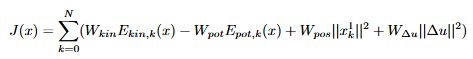
To make the controller solve the pendulum problem regardless of the angle of the pole (and to set it up for double pendulum in the future), I would like to set up the cost function to minimize the kinetic energy, maximize the potential energy, with setpoint tracking on the x position, and move suppression:
System Model
Code
def pendulum_ode_model(m_cart, mp1, l1, g=9.81, b_c=0.0, b_p=0.05) -> AcadosModel:
    model_name = 'pendulum'

    # constants
    m_cart = m_cart  # mass of the cart [kg]
    m = mp1  # mass of the ball [kg]
    g = g  # gravity constant [m/s^2]
    l = l1  # length of the rod [m]
    b_c = b_c  # friction coefficient for the cart
    b_p = b_p  # friction coefficient for the pendulum

    # set up states & controls
    x1      = SX.sym('x1')
    theta   = SX.sym('theta')
    v1      = SX.sym('v1')
    dtheta  = SX.sym('dtheta')
    u_prev  = SX.sym('u_prev')

    x = vertcat(x1, theta, v1, dtheta, u_prev)

    F = SX.sym('F')
    u = vertcat(F)

    # xdot
    x1_dot      = SX.sym('x1_dot')
    theta_dot   = SX.sym('theta_dot')
    v1_dot      = SX.sym('v1_dot')
    dtheta_dot  = SX.sym('dtheta_dot')
    u_prev_dot  = SX.sym('u_prev_dot')

    xdot = vertcat(x1_dot, theta_dot, v1_dot, dtheta_dot, u_prev_dot)

    # dynamics
    cos_theta = cos(theta)
    sin_theta = sin(theta)
    denominator = m_cart + m - m*cos_theta*cos_theta
    f_expl = vertcat(v1,
                     dtheta,
                     (-m*l*sin_theta*dtheta*dtheta + m*g*cos_theta*sin_theta + F - b_c*v1)/denominator,
                     (-m*l*cos_theta*sin_theta*dtheta*dtheta + F*cos_theta + (m_cart+m)*g*sin_theta - b_p*dtheta)/(l*denominator),
                     F
                     )

    f_impl = xdot - f_expl

    model = AcadosModel()

    model.f_impl_expr = f_impl
    model.f_expl_expr = f_expl
    model.x = x
    model.xdot = xdot
    model.u = u
    # model.z = u_prev
    model.name = model_name

    # add potential and kinetic energy expressions
    E_kin_cart = 1 / 2 * m_cart * v1**2
    E_kin_pendulum = 1 / 2 * m * ((v1 + l * dtheta * cos(theta))**2 + (l * dtheta * sin(theta))**2) + 1 / 2 * (m * l**2 / 3) * dtheta**2
    E_kin = E_kin_cart + E_kin_pendulum

    E_pot = m * g * l * cos(theta)

    model.E_kin = E_kin
    model.E_pot = E_pot

    # store meta information
    model.x_labels = ['$x$ [m]', r'$\theta$ [rad]', '$v$ [m]', r'$\dot{\theta}$ [rad/s]', '$u_{prev}$ [N]']
    model.u_labels = ['$F$']
    model.t_label = '$t$ [s]'

    return model
Following the example in the acados repo, I was able to formulate the NMPC with a NONLINEAR_LS cost function, as can be seen in this code:
Code
def formulate_pendulum_sim(model: AcadosModel,
                           dt: float = 0.05) -> AcadosSimSolver:
    """
    Construct the simulator/integrator for the plant model.
    """
    model.name += '_plant_sim'
    sim = AcadosSim()
    sim.model = model
    sim.solver_options.T = dt
    sim.solver_options.integrator_type = 'IRK'
    sim.solver_options.num_stages = 4
    sim.solver_options.num_steps = 3
    sim.solver_options.newton_iter = 3
    sim.solver_options.collocation_type = 'GAUSS_LEGENDRE'
    sim_solver = AcadosSimSolver(sim)
    return sim_solver

def formulate_pendulum_mpc(model: AcadosModel, N: int = 20, Tf: float = 1.0, RTI: bool = False,
                                Q: np.ndarray = np.diag([1e3, 1e3, 1e-2, 1e-2]),
                                Q_e: np.ndarray = np.diag([1e3, 1e3, 1e-2, 1e-2]),
                                cost_type: str = 'NONLINEAR_LS',
                                use_energy: bool = True,
                                x0: np.ndarray = np.array([0.0, np.pi, 0.0, 0.0]),
                                u_min: np.ndarray = np.array([-10.0]),
                                u_max: np.ndarray = np.array([10.0]),
                                x_min: np.ndarray = np.array([-0.7, -np.inf, -np.inf, -np.inf]),
                                x_max: np.ndarray = np.array([0.7, np.inf, np.inf, np.inf])
                                ) -> AcadosOcp:
    """
    Formulate the MPC problem for the pendulum model.
    """
    ocp = AcadosOcp()
    ocp.model = model
    ocp.solver_options.N_horizon = N
    ocp.solver_options.tf = Tf

    nx = model.x.rows()
    nu = model.u.rows()
    ny = nx + nu
    ny_e = nx
    x = ocp.model.x
    u = ocp.model.u
    E_kin = ocp.model.E_kin
    E_pot = ocp.model.E_pot
    u_prev = x[-1]

    if cost_type == 'NONLINEAR_LS':
        # Nonlinear least squares cost using kinetic and potential energy, cart position, and move suppression
        ocp.cost.cost_type = cost_type
        ocp.cost.cost_type_e = cost_type
        ocp.solver_options.hessian_approx = 'GAUSS_NEWTON'
        if use_energy:
            ocp.model.cost_y_expr = ca.vertcat(E_kin, -E_pot, x[0], (u - u_prev))
            ocp.model.cost_y_expr_e = ca.vertcat(E_kin, -E_pot, x[0], 0.0)
            n_ref = ocp.model.cost_y_expr.rows()
            ocp.cost.cost_type = cost_type
            ocp.cost.W = Q
            ocp.cost.W_e = Q_e
            ocp.cost.yref = np.zeros((n_ref,))
            ocp.cost.yref_e = np.zeros((n_ref,))
        else:
            ocp.model.cost_y_expr = ca.vertcat(x[:-1], u - u_prev)
            ocp.model.cost_y_expr_e = x[:-1]
            ocp.cost.W = Q
            ocp.cost.W_e = Q_e
            n_ref = ocp.model.cost_y_expr.rows()
            n_ref_e = ocp.model.cost_y_expr_e.rows()
            ocp.cost.yref = np.zeros((n_ref,))
            ocp.cost.yref_e = np.zeros((n_ref_e,))
    elif cost_type == 'EXTERNAL':
        # External cost function
        ocp.cost.cost_type = cost_type
        ocp.cost.cost_type_e = cost_type
        # Set up the external cost function
        ocp.model.cost_expr_ext_cost = Q[0,0] * E_kin + Q[1,1] * (-E_pot) + Q[2,2] * (ocp.model.x[0]**2) + Q[3,3] * (u - u_prev)**2
        ocp.model.cost_expr_ext_cost_e = Q_e[0,0] * E_kin + Q_e[1,1] * (-E_pot) + Q_e[2,2] * ocp.model.x[0]**2
        ext_cost_use_num_hess = False  # use numerical Hessian for external cost
        ocp.solver_options.ext_cost_num_hess = ext_cost_use_num_hess
        ocp.solver_options.hessian_approx = 'EXACT'
        ocp.solver_options.globalization_alpha_min = 1e-25


    # set constraints
    ocp.constraints.lbu = u_min
    ocp.constraints.ubu = u_max
    ocp.constraints.idxbu = np.arange(nu)

    ocp.constraints.lbx = x_min
    ocp.constraints.ubx = x_max
    ocp.constraints.idxbx = np.arange(nx)

    ocp.constraints.x0 = x0

    ocp.solver_options.qp_solver = 'FULL_CONDENSING_HPIPM'
    ocp.solver_options.qp_solver = 'PARTIAL_CONDENSING_HPIPM'
    # ocp.solver_options.qp_solver = 'PARTIAL_CONDENSING_OSQP'
    # ocp.solver_options.qp_solver = 'FULL_CONDENSING_QPOASES'
    ocp.solver_options.integrator_type = 'IRK'
    ocp.solver_options.nlp_solver_type = 'SQP' # SQP_RTI
    # ocp.solver_options.sim_method_num_steps = 10
    ocp.solver_options.sim_method_newton_iter = 5
    ocp.solver_options.tol = 1e-12
    # ocp.solver_options.tol = 1e-5
    # ocp.solver_options.sim_method_newton_tol = 1e-5
    ocp.solver_options.qp_solver_cond_N = N

    if RTI:
        ocp.solver_options.nlp_solver_type = 'SQP_RTI'
    else:
        ocp.solver_options.nlp_solver_type = 'SQP'
        ocp.solver_options.qp_solver_iter_max = 5000
        ocp.solver_options.nlp_solver_max_iter = 5000
        ocp.solver_options.globalization = 'MERIT_BACKTRACKING'

    solver_json = 'acados_ocp_' + model.name + '.json'
    acados_ocp_solver = AcadosOcpSolver(ocp, json_file = solver_json)
    return acados_ocp_solver
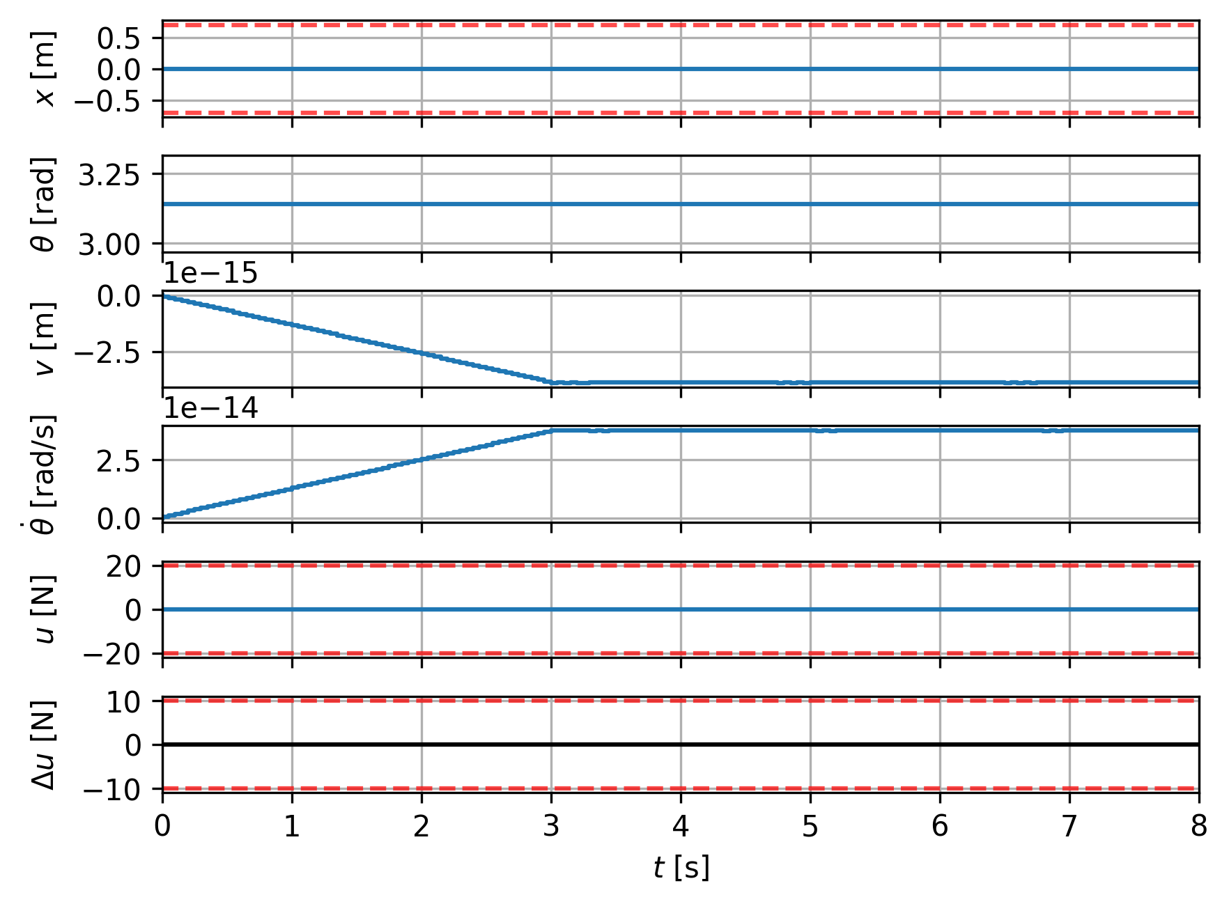
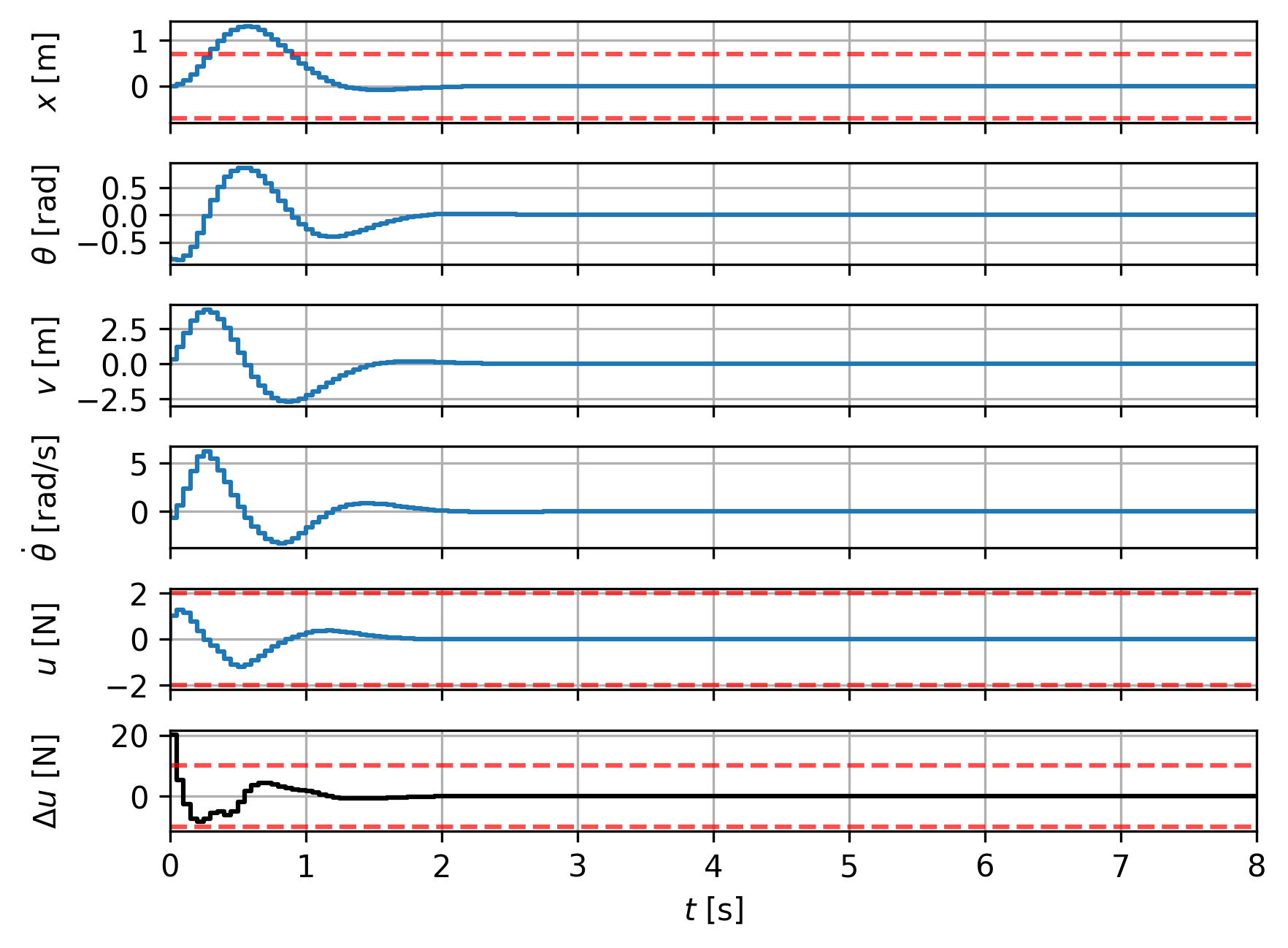
This formulation does not really follow the objective function presented at the top. More importantly, it seems that there are some robustness issues when utilizing this NONLINEAR_LS cost function. I noticed this as running the optimizer with SQP_RTI works well for all initial conditions, but this is not the case using just SQP. I also run into robustness issues when there is a slight plant-model mismatch or measurement noise.
The code above also includes my attempt at setting up an EXTERNAL cost function, which has not been successful thus far. Whenever I run it with the EXTERNAL cost, I end up with the following message:
SQP_RTI: QP solver returned error status 3 QP iteration 15.
The controller does not make any significant moves in the manipulated variable with the EXTERNAL cost function set up. I tried reducing globalization_alpha_min but that does not seem to fix the issue. I also tried using different weights with no luck.
NMPC Setup in main.py
Code
def main():
    # Define parameters
    m_cart = 0.035  # mass of the cart [kg]
    mp1 = 0.034  # mass of the pendulum [kg]
    l1 = 0.25  # length of the rod [m]
    g = 9.81  # gravity constant [m/s^2]
    b_c = 0.0  # friction coefficient for the cart
    b_p = 0.0  # friction coefficient for the pendulum

    Tsim = 8.0  # final time for simulation [s]
    dt = 0.025  # time step for simulation [s] and sampling time for the ocp
    Nsim = int(Tsim / dt)  # number of steps
    Tf = 1.0 # length of the prediction horizon [s]
    N_horizon = int(Tf/dt)  # MPC number of stages in the prediction horizon

    # get the pendulum model
    model = pendulum_ode_model(m_cart, mp1, l1, g, b_c, b_p)
    nx = model.x.rows()  # number of states
    nu = model.u.rows()  # number of controls

    # Initiate simulation integrator
    sim_solver = formulate_pendulum_sim(model, dt=dt)

    # Formulate the MPC controller as an OCP solver
    cost_type = 'EXTERNAL'  # cost type
    # cost_type = 'EXTERNAL'  # cost type for external cost function
    RTI = True  # Real-Time Iteration
    use_energy = True  # use energy in the cost function

    if cost_type == 'NONLINEAR_LS':
        if use_energy:
            Q = 200*np.diag([1.0, 30.0, 1.0, 0.6])  # output reference tracking cost matrix
            Q_e = 200*np.diag([1.0, 15.0, 0.75, 0])  # terminal output reference tracking cost matrix
        else:
            Q = 2*np.diag([1e2, 1e2, 0, 0, 4e-1])  # state reference tracking cost matrix
            Q_e = 2*np.diag([1e2, 1e2, 0, 0]) # terminal state reference tracking cost matrix
    elif cost_type == 'EXTERNAL':
        Q = 200*np.diag([1.0, 10.0, 15.0, 0.7])  # weights for the external cost function
        Q_e = 200*np.diag([1.0, 1.0, 0.75, 0])  # terminal weights for the external cost function

    x0 = np.array([0.0, 1*np.pi, 0.0, 0.0, 0.0])  # initial state [x1, theta, v1, dtheta, u_prev]
    u_min = np.array([-2.0])  # minimum control input
    u_max = np.array([2.0])  # maximum control input
    x_min = np.array([-0.5, -ACADOS_INFTY, -ACADOS_INFTY, -ACADOS_INFTY, -ACADOS_INFTY])  # minimum state
    x_max = np.array([0.5, ACADOS_INFTY, ACADOS_INFTY, ACADOS_INFTY, ACADOS_INFTY])     # maximum state
    controller_config = {
        'N': N_horizon,  # number of stages in the prediction horizon
        'Tf': Tf,  # length of the prediction horizon [s]
        'Q': Q,  # state cost matrix
        'Q_e': Q_e,  # terminal state cost matrix
        'x0': x0,  # initial state
        'u_min': u_min,  # minimum control input
        'u_max': u_max,   # maximum control input
        'x_min': x_min,  # minimum state
        'x_max': x_max,  # maximum state
        'cost_type': cost_type,  # cost type
        'RTI': RTI,  # Real-Time Iteration
        'use_energy': use_energy,  # use energy in the cost function
    }
    mpc = formulate_pendulum_mpc(model, **controller_config)
Questions
Is there anything I am missing or overlooking in my code, especially for the EXTERNAL cost set up?
Are there any additional examples for EXTERNAL cost set up that can help guide me with this project?
Could the numerical issues cause the lack of robustness in the NONLINEAR_LS cost formulation (the masses of my 3D printed setup in the lab are quite low)? and if so, would adjusting the scaling result in more robust NMPC?
Thank you for your advice! ![]()