Here’s the original code:
F8_crusader_model
function model = F8_crusader_model()
import casadi.*

%% System dimension
nx = 3;
nu = 1;

%% System parameters
a1 = -0.877; a2 = -0.088; a3 = 0.47; a4 = -0.019; a5 = 3.846; a6 = -0.215;
a7 = 0.28; a8 = 0.47; a9 = 0.63;
c1 = -4.208; c2 = -0.396; c3 = -0.47; c4 = -3.564; c5 = -20.967; c6 = 6.265;
c7 = 46; c8 = 61.1;

%% Symbolic variables
% states
x1 = SX.sym('x1');
x2 = SX.sym('x2');
x3 = SX.sym('x3');
sym_x = vertcat(x1, x2, x3);

% controls
u = SX.sym('u');
sym_u = u;

% state derivatives
sym_xdot = SX.sym('xdot', nx, 1);

%% The system dynamics
% Explicit Dynamics
expr_f_expl = vertcat(a1*x1+x3+a2*x1*x3+a3*x1.^2+a4*x2.^2-x1.^2*x3+a5*x1.^3+a6*u+a7*x1.^2*u+a8*x1*u.^2+a9*u.^3, ...
                      x3, ...
                      c1*x1+c2*x3+c3*x1.^2+c4*x1.^3+c5*u+c6*x1.^2*u+c7*x1*u.^2+c8*u.^3);

% Implicit Dynamics
expr_f_impl = expr_f_expl - sym_xdot;

% Discrete Dynamics

%% fill structure
model.nx = nx;
model.nu = nu;
model.sym_x = sym_x;
model.sym_u = sym_u;
model.sym_xdot = sym_xdot;
model.expr_f_expl = expr_f_expl;
model.expr_f_impl = expr_f_impl;

end
F8_crusader_ocp
%% Test of native matlab interface
clear; close all; clc;

% run acados_env_variables_windows.m
run('../acados_env_variables_windows.m');

% check that env.sh has been run
env_run = getenv('ENV_RUN');
if (~strcmp(env_run, 'true'))
	error('env.sh has not been sourced! Before executing this example, run: source env.sh');
end

%% Solver options
% Code generation
compile_interface = 'false';
codgen_model = 'false';
compile_model = 'false';
output_dir = 'build';

% Shooting nodes
param_scheme_N = 10;                     % horizon parameter (need T)

% Integrator
sim_method = 'erk';
sim_method_num_stages = 4;
sim_method_num_steps = 1;
% sim_method_newton_iter = 3;            % for 'irk' 'irk_gnsf'
gnsf_detect_struct = 'true';

% NLP solver
nlp_solver = 'sqp_rti';
nlp_solver_max_iter = 100;
nlp_solver_tol_stat = 10e-6;
nlp_solver_tol_eq = 10e-6;
nlp_solver_tol_ineq = 10e-6;
nlp_solver_tol_comp = 10e-6;
nlp_solver_ext_qp_res = 0;               % for debugging
nlp_solver_step_length = 1.0;
rti_phase = 0;                           % for sqp_rti

% QP solver
qp_solver = 'partial_condensing_hpipm';
qp_solver_iter_max = 50;
qp_solver_cond_N = 5;                    % for partial_condensing
qp_solver_cond_ric_alg = 1;
qp_solver_ric_alg = 1;                   % for HPIPM
qp_solver_warm_start = 0;
% warm_start_first_qp = 1;

% Globalization
globalization = 'fixed_step';
% alpha_min = 0.05;                      % for merit_backtracking
% alpha_reduction = 0.7;

% Hessian approximation
nlp_solver_exact_hessian = 'false';      % 'gauss newton'
regularize_method = 'no_regularize';
levenberg_marquardt = 0.0;
% exact_hess_dyn = 1;                    % for exact_hessian = 'true'
% exact_hess_cost = 1;
% exact_hess_constr = 1;

% Other
print_level = 0;

%% OCP options

% model_name = 'F8_crusader';

% CasADi expression
model = F8_crusader_model;

% time horizon length
h = 0.01;
T = param_scheme_N*h;

% dimension
nx = model.nx;
nu = model.nu;
ny = nx + nu;                  % number of outputs in lagrange term
ny_e = nx;                     % number of outputs in mayer term
nbx = nx;                      % number of state bounds
nbu = nu;                      % number of input bounds

% cost
cost_type = 'linear_ls';
cost_type_e = 'linear_ls';
Vx = zeros(ny,nx); Vx(1:nx,:) = eye(nx);        % state-to-output matrix in lagrange term
Vu = zeros(ny,nu); Vu(nx+1:ny,:) = eye(nu);     % input-to-output matrix in lagrange term
Vx_e = zeros(ny_e,nx); Vx_e(1:nx,:) = eye(nx);  % state-to-output matrix in mayer term
W = diag([25*2, 0, 0, 0.05*2]);
W_e = W(1:ny_e,1:ny_e);
y_ref = zeros(ny,1);                            % set intial references
y_ref_e = zeros(ny_e,1);

% constraint
constr_type = 'bgh';
dyn_type = 'explicit';
x0 = [0.1; 0; 0];
Jbx = eye(nbx,nx);
lbx = [-0.2; -1; -1];
ubx = [0.4; 1; 1];
Jbu = eye(nbu,nu);
lbu = -0.3;
ubu = 0.5;

%% acados ocp model
ocp_model = acados_ocp_model();
% ocp_model.set('name', model_name);

% end time
ocp_model.set('T', T);

% symbolics
ocp_model.set('sym_x', model.sym_x);
ocp_model.set('sym_u', model.sym_u);
ocp_model.set('sym_xdot', model.sym_xdot);

% cost
ocp_model.set('cost_type', cost_type);
ocp_model.set('cost_type_e', cost_type_e);
ocp_model.set('cost_Vx', Vx);
ocp_model.set('cost_Vu', Vu);
ocp_model.set('cost_Vx_e', Vx_e);
ocp_model.set('cost_W', W);
ocp_model.set('cost_W_e', W_e);
ocp_model.set('cost_y_ref', y_ref);
ocp_model.set('cost_y_ref_e', y_ref_e);

% constraint
ocp_model.set('dyn_type', dyn_type);
ocp_model.set('dyn_expr_f', model.expr_f_expl);
ocp_model.set('constr_x0', x0);                 % dynamic
ocp_model.set('constr_type', constr_type);
ocp_model.set('constr_Jbx', Jbx);
ocp_model.set('constr_lbx', lbx);
ocp_model.set('constr_ubx', ubx);
ocp_model.set('constr_Jbu', Jbu);
ocp_model.set('constr_lbu', lbu);
ocp_model.set('constr_ubu', ubu);

disp('ocp_model.model_struct: ')
disp(ocp_model.model_struct)

%% acados ocp opts
ocp_opts = acados_ocp_opts();

% Code generation
ocp_opts.set('compile_interface', compile_interface);
ocp_opts.set('codgen_model', codgen_model);
ocp_opts.set('compile_model', compile_model);
ocp_opts.set('output_dir', output_dir);

% Shooting nodes
ocp_opts.set('param_scheme_N', param_scheme_N);

% Integrator
ocp_opts.set('sim_method', sim_method);
ocp_opts.set('sim_method_num_stages', sim_method_num_stages);
ocp_opts.set('sim_method_num_steps', sim_method_num_steps);
% ocp_opts.set('sim_method_newton_iter', sim_method_newton_iter);
ocp_opts.set('gnsf_detect_struct', gnsf_detect_struct);

% NLP solver
ocp_opts.set('nlp_solver', nlp_solver);
ocp_opts.set('qp_solver_iter_max', qp_solver_iter_max);
ocp_opts.set('nlp_solver_tol_stat', nlp_solver_tol_stat);
ocp_opts.set('nlp_solver_tol_eq', nlp_solver_tol_eq);
ocp_opts.set('nlp_solver_tol_ineq', nlp_solver_tol_ineq);
ocp_opts.set('nlp_solver_tol_comp', nlp_solver_tol_comp);
ocp_opts.set('nlp_solver_ext_qp_res', nlp_solver_ext_qp_res);
ocp_opts.set('nlp_solver_step_length', nlp_solver_step_length);
ocp_opts.set('rti_phase', rti_phase);

% QP solver
ocp_opts.set('qp_solver', qp_solver);
ocp_opts.set('qp_solver_iter_max', qp_solver_iter_max);
ocp_opts.set('qp_solver_cond_N', qp_solver_cond_N);
ocp_opts.set('qp_solver_cond_ric_alg', qp_solver_cond_ric_alg);
ocp_opts.set('qp_solver_ric_alg', qp_solver_ric_alg);
ocp_opts.set('qp_solver_warm_start', qp_solver_warm_start);
% ocp_opts.set('nlp_solver_warm_start_first_qp', warm_start_first_qp);

% Globalization
ocp_opts.set('globalization', globalization);
% ocp_opts.set('alpha_min', alpha_min);
% ocp_opts.set('alpha_reduction', alpha_reduction);

% Hessian approximation
ocp_opts.set('nlp_solver_exact_hessian', nlp_solver_exact_hessian);
ocp_opts.set('regularize_method', regularize_method);
ocp_opts.set('levenberg_marquardt', levenberg_marquardt);
% ocp_opts.set('exact_hess_dyn', exact_hess_dyn);
% ocp_opts.set('exact_hess_cost', exact_hess_cost);
% ocp_opts.set('exact_hess_constr', exact_hess_constr);

% Other
ocp_opts.set('print_level', print_level);

disp('ocp_opts.opts_struct: ');
disp(ocp_opts.opts_struct);

%% create ocp solver
ocp = acados_ocp(ocp_model, ocp_opts);

%% Simulation
Duration = 10;
N_sim = Duration/h;

% initialize data structs
x_sim = zeros(nx, N_sim+1);
u_sim = zeros(nu, N_sim+1);
cost_sim = zeros(1, N_sim+1);
x_sim(:, 1) = x0;
u_sim(:, 1) = zeros(nu, 1);
cost_sim(1, 1) = 0;

% set trajectory initialization (also can use plant: create acados integrator)
ocp.set('init_x', x0 * ones(1,param_scheme_N+1));
% ocp.set('init_x', zeros(nx,param_scheme_N+1));
ocp.set('init_u', zeros(nu, param_scheme_N));

% time-varying reference trajectory
x1ref_FUN = @(t) 0.4.*(-(0.5./(1+exp(t./0.1-0.8))) + (1./(1+exp(t./0.1-30))) - 0.4);
t = 0:h:Duration;
x1ref = 0.4.*(-(0.5./(1+exp(t./0.1-0.8))) + (1./(1+exp(t./0.1-30))) - 0.4);

% run mpc
fprintf('Simulation started.  It might take a while...\n')
tic;
for i = 1:N_sim

    % update reference
    t_ref = (i-1:i+param_scheme_N).*h;
    x1_ref = x1ref_FUN(t_ref);
    for j = 0:param_scheme_N-1
        y_ref(1) = x1_ref(j+1);
        ocp.set('cost_y_ref', y_ref, j);
    end
    y_ref_e(1) = x1_ref(param_scheme_N+1);
    ocp.set('cost_y_ref_e', y_ref_e, param_scheme_N);

    % solve ocp
    ocp.solve();
    status = ocp.get('status');      % 0 - success
    if status ~= 0
        error(sprintf('acados returned status %d in closed loop iteration %d. Exiting.', status, i));
    end

    % get solution t0
    x0 = ocp.get('x', 0);
    u0 = ocp.get('u', 0);
    x_sim(:, i+1) = x0;
    u_sim(:, i+1) = u0;
    cost_sim(1, i+1) = ocp.get_cost();

    % update initial state
    x0 = ocp.get('x', 1);
    ocp.set('constr_x0', x0);

end
tElapsed = toc
fprintf('Simulation finished!\n')

%% Plot
figure; hold on; grid on;
plot(t, x_sim, t, x1ref, '--');
legend('x1', 'x2', 'x3', 'x1Ref');

figure; hold on; grid on;
plot(t, u_sim);
legend('the control input');

figure; hold on; grid on;
plot(t, cost_sim);
legend('the cost curve');

%% go embedded to generate templated C code
% ocp.generate_c_code;
Here’s the code using augmented state variables:
F8_crusader_model
function model = F8_crusader_model()
import casadi.*

%% System dimension
nx = 4;
nu = 1;

%% System parameters
a1 = -0.877; a2 = -0.088; a3 = 0.47; a4 = -0.019; a5 = 3.846; a6 = -0.215;
a7 = 0.28; a8 = 0.47; a9 = 0.63;
c1 = -4.208; c2 = -0.396; c3 = -0.47; c4 = -3.564; c5 = -20.967; c6 = 6.265;
c7 = 46; c8 = 61.1;

%% Symbolic variables
% states
x1 = SX.sym('x1');
x2 = SX.sym('x2');
x3 = SX.sym('x3');
x4 = SX.sym('x4');
sym_x = vertcat(x1, x2, x3, x4);

% controls
u = SX.sym('u');
sym_u = u;

% state derivatives
sym_xdot = SX.sym('xdot', nx, 1);

%% The system dynamics
% Explicit Dynamics
expr_f_expl = vertcat(a1*x1+x3+a2*x1*x3+a3*x1.^2+a4*x2.^2-x1.^2*x3+a5*x1.^3+a6*x4+a7*x1.^2*x4+a8*x1*x4.^2+a9*x4.^3, ...
                      x3, ...
                      c1*x1+c2*x3+c3*x1.^2+c4*x1.^3+c5*x4+c6*x1.^2*x4+c7*x1*x4.^2+c8*x4.^3, ...
                      u);

% Implicit Dynamics
expr_f_impl = expr_f_expl - sym_xdot;

% Discrete Dynamics

%% fill structure
model.nx = nx;
model.nu = nu;
model.sym_x = sym_x;
model.sym_u = sym_u;
model.sym_xdot = sym_xdot;
model.expr_f_expl = expr_f_expl;
model.expr_f_impl = expr_f_impl;

end
F8_crusader_ocp
%% Test of native matlab interface
clear; close all; clc;
% run acados_env_variables_windows.m
run('../acados_env_variables_windows.m');
% check that env.sh has been run
env_run = getenv('ENV_RUN');
if (~strcmp(env_run, 'true'))
error('env.sh has not been sourced! Before executing this example, run: source env.sh');
end
%% Solver options
% Code generation
compile_interface = 'false';
codgen_model = 'false';
compile_model = 'false';
output_dir = 'build';
% Shooting nodes
param_scheme_N = 10; % horizon parameter (need T)
% Integrator
sim_method = 'erk';
sim_method_num_stages = 4;
sim_method_num_steps = 1;
% sim_method_newton_iter = 3; % for 'irk' 'irk_gnsf'
gnsf_detect_struct = 'true';
% NLP solver
nlp_solver = 'sqp_rti';
nlp_solver_max_iter = 100;
nlp_solver_tol_stat = 10e-6;
nlp_solver_tol_eq = 10e-6;
nlp_solver_tol_ineq = 10e-6;
nlp_solver_tol_comp = 10e-6;
nlp_solver_ext_qp_res = 0; % for debugging
nlp_solver_step_length = 1.0;
rti_phase = 0; % for sqp_rti
% QP solver
qp_solver = 'partial_condensing_hpipm';
qp_solver_iter_max = 50;
qp_solver_cond_N = 5; % for partial_condensing
qp_solver_cond_ric_alg = 1;
qp_solver_ric_alg = 1; % for HPIPM
qp_solver_warm_start = 1;
% warm_start_first_qp = 1;
% Globalization
globalization = 'fixed_step';
% alpha_min = 0.05; % for merit_backtracking
% alpha_reduction = 0.7;
% Hessian approximation
nlp_solver_exact_hessian = 'false'; % 'gauss newton'
regularize_method = 'no_regularize';
levenberg_marquardt = 0.0;
% exact_hess_dyn = 1; % for exact_hessian = 'true'
% exact_hess_cost = 1;
% exact_hess_constr = 1;
% Other
print_level = 0;
%% OCP options
% model_name = 'F8_crusader';
% CasADi expression
model = F8_crusader_model;
% time horizon length
h = 0.01;
T = param_scheme_N*h;
% dimension
nx = model.nx;
nu = model.nu;
ny = nx + nu; % number of outputs in lagrange term
ny_e = nx; % number of outputs in mayer term
nbx = nx; % number of state bounds
nbu = nu; % number of input bounds
% cost
cost_type = 'linear_ls';
cost_type_e = 'linear_ls';
Vx = zeros(ny,nx); Vx(1:nx,:) = eye(nx); % state-to-output matrix in lagrange term
Vu = zeros(ny,nu); Vu(nx+1:ny,:) = eye(nu); % input-to-output matrix in lagrange term
Vx_e = zeros(ny_e,nx); Vx_e(1:nx,:) = eye(nx); % state-to-output matrix in mayer term
W = diag([5*2, 0, 0, 0.5*2, 0.05*2]);
W_e = W(1:ny_e,1:ny_e);
y_ref = zeros(ny,1); % set intial references
y_ref_e = zeros(ny_e,1);
% constraint
constr_type = 'bgh';
dyn_type = 'explicit';
x0 = [0.1; 0; 0; 0];
Jbx = eye(nbx,nx);
lbx = [-0.2; -1; -1; -0.3];
ubx = [0.4; 1; 1; 0.5];
Jbu = eye(nbu,nu);
lbu = -0.3;
ubu = 0.5;
%% acados ocp model
ocp_model = acados_ocp_model();
% ocp_model.set('name', model_name);
% end time
ocp_model.set('T', T);
% symbolics
ocp_model.set('sym_x', model.sym_x);
ocp_model.set('sym_u', model.sym_u);
ocp_model.set('sym_xdot', model.sym_xdot);
% cost
ocp_model.set('cost_type', cost_type);
ocp_model.set('cost_type_e', cost_type_e);
ocp_model.set('cost_Vx', Vx);
ocp_model.set('cost_Vu', Vu);
ocp_model.set('cost_Vx_e', Vx_e);
ocp_model.set('cost_W', W);
ocp_model.set('cost_W_e', W_e);
ocp_model.set('cost_y_ref', y_ref);
ocp_model.set('cost_y_ref_e', y_ref_e);
% constraint
ocp_model.set('dyn_type', dyn_type);
ocp_model.set('dyn_expr_f', model.expr_f_expl);
ocp_model.set('constr_x0', x0); % dynamic
ocp_model.set('constr_type', constr_type);
ocp_model.set('constr_Jbx', Jbx);
ocp_model.set('constr_lbx', lbx);
ocp_model.set('constr_ubx', ubx);
ocp_model.set('constr_Jbu', Jbu);
ocp_model.set('constr_lbu', lbu);
ocp_model.set('constr_ubu', ubu);
disp('ocp_model.model_struct: ')
disp(ocp_model.model_struct)
%% acados ocp opts
ocp_opts = acados_ocp_opts();
% Code generation
ocp_opts.set('compile_interface', compile_interface);
ocp_opts.set('codgen_model', codgen_model);
ocp_opts.set('compile_model', compile_model);
ocp_opts.set('output_dir', output_dir);
% Shooting nodes
ocp_opts.set('param_scheme_N', param_scheme_N);
% Integrator
ocp_opts.set('sim_method', sim_method);
ocp_opts.set('sim_method_num_stages', sim_method_num_stages);
ocp_opts.set('sim_method_num_steps', sim_method_num_steps);
% ocp_opts.set('sim_method_newton_iter', sim_method_newton_iter);
ocp_opts.set('gnsf_detect_struct', gnsf_detect_struct);
% NLP solver
ocp_opts.set('nlp_solver', nlp_solver);
ocp_opts.set('qp_solver_iter_max', qp_solver_iter_max);
ocp_opts.set('nlp_solver_tol_stat', nlp_solver_tol_stat);
ocp_opts.set('nlp_solver_tol_eq', nlp_solver_tol_eq);
ocp_opts.set('nlp_solver_tol_ineq', nlp_solver_tol_ineq);
ocp_opts.set('nlp_solver_tol_comp', nlp_solver_tol_comp);
ocp_opts.set('nlp_solver_ext_qp_res', nlp_solver_ext_qp_res);
ocp_opts.set('nlp_solver_step_length', nlp_solver_step_length);
ocp_opts.set('rti_phase', rti_phase);
% QP solver
ocp_opts.set('qp_solver', qp_solver);
ocp_opts.set('qp_solver_iter_max', qp_solver_iter_max);
ocp_opts.set('qp_solver_cond_N', qp_solver_cond_N);
ocp_opts.set('qp_solver_cond_ric_alg', qp_solver_cond_ric_alg);
ocp_opts.set('qp_solver_ric_alg', qp_solver_ric_alg);
ocp_opts.set('qp_solver_warm_start', qp_solver_warm_start);
% ocp_opts.set('nlp_solver_warm_start_first_qp', warm_start_first_qp);
% Globalization
ocp_opts.set('globalization', globalization);
% ocp_opts.set('alpha_min', alpha_min);
% ocp_opts.set('alpha_reduction', alpha_reduction);
% Hessian approximation
ocp_opts.set('nlp_solver_exact_hessian', nlp_solver_exact_hessian);
ocp_opts.set('regularize_method', regularize_method);
ocp_opts.set('levenberg_marquardt', levenberg_marquardt);
% ocp_opts.set('exact_hess_dyn', exact_hess_dyn);
% ocp_opts.set('exact_hess_cost', exact_hess_cost);
% ocp_opts.set('exact_hess_constr', exact_hess_constr);
% Other
ocp_opts.set('print_level', print_level);
disp('ocp_opts.opts_struct: ');
disp(ocp_opts.opts_struct);
%% create ocp solver
ocp = acados_ocp(ocp_model, ocp_opts);
%% Simulation
Duration = 10;
N_sim = Duration/h;
% initialize data structs
x_sim = zeros(nx, N_sim+1);
u_sim = zeros(nu, N_sim+1);
cost_sim = zeros(1, N_sim+1);
x_sim(:, 1) = x0;
u_sim(:, 1) = zeros(nu, 1);
cost_sim(1, 1) = 0;
% set trajectory initialization (also can use plant: create acados integrator)
ocp.set('init_x', x0 * ones(1,param_scheme_N+1));
% ocp.set('init_x', zeros(nx,param_scheme_N+1));
ocp.set('init_u', zeros(nu, param_scheme_N));
% time-varying reference trajectory
x1ref_FUN = @(t) 0.4.*(-(0.5./(1+exp(t./0.1-0.8))) + (1./(1+exp(t./0.1-30))) - 0.4);
t = 0:h:Duration;
x1ref = 0.4.*(-(0.5./(1+exp(t./0.1-0.8))) + (1./(1+exp(t./0.1-30))) - 0.4);
% run mpc
fprintf('Simulation started. It might take a while...\n')
tic;
for i = 1:N_sim
% update reference
t_ref = (i-1:i+param_scheme_N).*h;
x1_ref = x1ref_FUN(t_ref);
for j = 0:param_scheme_N-1
y_ref(1) = x1_ref(j+1);
ocp.set('cost_y_ref', y_ref, j);
end
y_ref_e(1) = x1_ref(param_scheme_N+1);
ocp.set('cost_y_ref_e', y_ref_e, param_scheme_N);
% solve ocp
ocp.solve();
status = ocp.get('status'); % 0 - success
if status ~= 0
error(sprintf('acados returned status %d in closed loop iteration %d. Exiting.', status, i));
end
% get solution t0
x0 = ocp.get('x', 0);
u0 = ocp.get('u', 0);
x_sim(:, i+1) = x0;
u_sim(:, i+1) = u0;
cost_sim(1, i+1) = ocp.get_cost();
% update initial state
x0 = ocp.get('x', 1);
ocp.set('constr_x0', x0);
end
tElapsed = toc
fprintf('Simulation finished!\n')
%% Plot
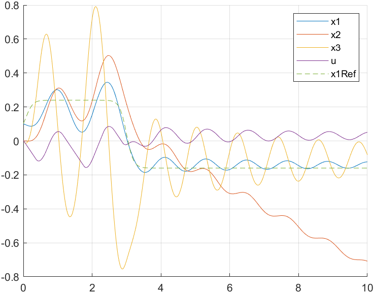
figure; hold on; grid on;
plot(t, x_sim, t, x1ref, '--');
legend('x1', 'x2', 'x3', 'u', 'x1Ref');
figure; hold on; grid on;
plot(t, u_sim);
legend('udot');
figure; hold on; grid on;
plot(t, cost_sim);
legend('the cost curve');
%% go embedded to generate templated C code
% ocp.generate_c_code;