Does acados support state times input dynamics?

Hello all,
First, thank you to all the people involved with this tool and the forum which has already been a great resource to resolve many of my issues.

Unfortunately I have not yet been able to find the answer for this particular issue. To clarify the question from the title:
Does acados support dynamic expressions where a state is multiplied by the input (decision variable), and if so, how? I think that this question sums up the issues I am having, and I’m starting off with this general question in case there is a quick and simple answer, but I’ll elaborate on the details with a reduced example below (apologies, it is a little lengthy still):

  1. I am using the Matlab interface of acados, but installed just before the recent overhaul which brought the syntax in line with the Python version.

  2. The exact problem I encounter is that I would like to control an algebraic state, z1, to a reference value. This state is defined as z1 = u * x1, which is the multiplication of the system input, u, and a system state, x1. Unfortunately, I can’t get that to work. (I am using the implicit dynamics mode, more details in point 4 below)

  3. Where I believe my problem comes from: The projected trajectory of the algebraic state, z1, acquired from the solved ocp does not match the defined system behavior. The trajectory after solving the ocp, which is acquired via ocp.get('z'), does not match the trajectory that I can calculate by multiplying the inputs and states, u * x1, acquired from ocp.get('u') and ocp.get('x'). This plot shows the difference between the two.
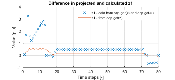
    z1_doesnt_match
    Given that this projected trajectory of z1 is incorrect, it is no surprise to me that tracking this to a reference value will not work well either. This is what leads me to ask whether such dynamics are even supported, or whether I am still setting something up incorrectly. Some additional points:

  • The trajectories from ocp.get('x') are correct, as I have verified them by applying the input trajectory to an external model.
  • When the system is in a more constant state the error is significantly reduced
  • Reducing the sampling time also reduces the error

From here on I will describe how I set up the solver:

  1. How I set up the ocp: I am using the implicit dynamics mode to specify the system dynamics as follows (in this case I’m using as a reduced example an averaged model of a DC/DC buck converter, where z1 denotes the input current):
f_impl = vertcat(- x1_dot + u * (p1/p2) - x2 * (1/p2), ...
                 x1 * (1/p3) - x2 * (1/(p4*p3)) - x2_dot,...
                 z1 - (u * x1));

Where the states/inputs/params are defined as:

% // States
% // Differential States (x vector)
x1 = SX.sym('x1');  % // inductor current
x2 = SX.sym('x2');  % // capacitor voltage output
x = vertcat(x1, x2); % // state vector

% //algebraic states (z vector)
z1 = SX.sym('z1');
z = vertcat(z1);

% ///inputs
u = SX.sym('u');  % duty cycle input

% //state derivatives (x dot vector)
x1_dot = SX.sym('x1_dot'); % derivative of inductor current
x2_dot = SX.sym('x2_dot'); % derivative of capacitor voltage
x_dot = vertcat(x1_dot, x2_dot); % state derivative vector

% //system parameters (constants so no need for expressions)
% //p1, p2, p3, p4
  1. I initially set up the ocp with the linear least squares cost type to track z1 to a reference value. When this wasn’t working I set it up to track x2 to a reference value instead for troubleshooting. This is the case in the plot shown above in point 3.
  • I have also tried to exclude z1 altogether and track the u * x1 using the non-linear least squares cost module. While this does tend to reach the reference value in a step response eventually, I believe it suffers from a similar issue of incorrect projections, but I have not been able to verify this as I don’t believe there is access to the actual cost of an optimized decision, is there?
  1. Model and ocp settings were largely taken from the example \acados\examples\acados_matlab_octave\pendulum_dae. At first I simply replaced the dynamic equation and states but in troubleshooting I have since then attempted most different integrator and solver settings with no luck.

Thank you to anyone who takes the time to read this, I hope you can shed some light on the situation!

(PS. I thought I had seen whole matlab script files in other posts but I haven’t been able to find those again and I haven’t yet figured out how to do it myself. If anyone would like the full script of the example I use here please let me know how to upload that :slight_smile: )

Hi :wave:

this sounds like your integrator is not converging. Try to set the solver option sim_method_newton_iter to something large, like 50, and sim_method_newton_tol to the tolerance you would like to have, e.g. 1e-6.

Hope this helps,
Katrin

Hello, thank your for the reply!

I’ve set the sim_method_newton_iter to 50, even 5000. It certainly takes longer to run but no change in results. The sim_method_newton_tol however does not appear to be a field I can set in the matlab interface (at least in the acados version I have, perhaps I should try with the most recent update?).

But based on your answer, can I safely assume that the input*state dynamic does not immediately strike you as an unsupported use case?

While I was not able to set the sim_method_newton_tol via the matlab interface, I found what I believe to the template files where the default value of is set.

In my case I found the files in C:\acados\interfaces\acados_matlab_octave\acados_template_mex\+acados_template_mex\AcadosOcpOptions.m and C:\acados\interfaces\acados_matlab_octave\acados_template_mex\+acados_template_mex\AcadosSim.m. (I hope this is what I think it is)

I changed the default value from 0.0 to 0.000001 in these files, which does seem to work as the .json which is generated when compiling the mex files now does have "sim_method_newton_tol":1e-06 in it.

Unfortunately, there is still no change in the error of my algebraic state :frowning: , so if it is the integrator not converging then these settings have not helped unfortunately.

On the topic of the integrator, these are the settings I use now incase this is useful information:

ocp_sim_method = 'irk';    % set the settings
ocp_sim_method_num_stages = 4 * ones(ocp_N, 1); 
ocp_sim_method_num_steps = 1; 
ocp_sim_method_newton_iter = 5000;  % <- tried different options here

ocp_opts.set('sim_method', ocp_sim_method); %put settings into the options
ocp_opts.set('sim_method_num_stages', ocp_sim_method_num_stages);
ocp_opts.set('sim_method_num_steps', ocp_sim_method_num_steps);
ocp_opts.set('sim_method_newton_iter', ocp_sim_method_newton_iter);
    

I have also tried different Runge-Kutta stages, also no improvement :frowning:

The dynamicsare fine in general. But the behaviour you describe seems indeed weird.

Is the solver converging for all of the problems, i.e. do you get status 0? If not could you provide the output of print_statistics?

As a next step I would recommend to test with the integrator separately (without the OCP).

If you can provide a minimal working example I can also have a look.

Yes, I do get status 0, using ocp.get('status') .

For the more detailed statistics, using ocp.print('stat') I get:

iter	qp_status	qp_iter
0	0		0
1	0		11

But I think it’s somewhat misaligned, 11 is the number of qp iterations. When running in a closed loop the only thing that changes in these stats is the number of qp iterations.

I have a minimal example with the OCP, not yet with integrator separately (I’ll be trying that out now).

Minimal example with OCP, ready to copy/paste into a matlab script and run:

% All in one file, minimal, for running simple MPC buck converter with acados
% implicit dynamics form
close all; clearvars; clear functions
%% Circuit Paramters - Per Unit Values
Rpu_load = 1;
Cpu_out = 97.9;
Lpu_out = 0.562;
Vpu_source = 1;
Tpu_sampling = 1;

%% Check
% check that env.sh has been run
env_run = getenv('ENV_RUN');
if (~strcmp(env_run, 'true'))
	error('env.sh has not been sourced! Before executing this example, run: source env.sh');
end

%% options
compile_interface = 'auto'; % true, false
codgen_model = 'true'; % true, false
model_name = 'buckConv_dae';

% ocp
ocp_N = 80; % prediction horizon
nlp_solver = 'sqp_rti'; % sqp, sqp_rti
nlp_solver_exact_hessian = 'false';
regularize_method = 'no_regularize'; % no_regularize, project,...
    % project_reduc_hess, mirror, convexify
nlp_solver_max_iter = 500;
qp_solver = 'full_condensing_hpipm';
        % full_condensing_hpipm, partial_condensing_hpipm
qp_solver_cond_N = 5;
qp_solver_warm_start = 0;
qp_solver_cond_ric_alg = 0; % 0: dont factorize hessian in the condensing; 1: factorize
qp_solver_ric_alg = 0; % HPIPM specific
ocp_sim_method = 'irk'; % irk, irk_gnsf
ocp_sim_method_num_stages = 2 * ones(ocp_N, 1); % scalar or vector of size ocp_N;
ocp_sim_method_num_steps = 1; % scalar or vector of size ocp_N;
ocp_sim_method_newton_iter = 5000; % make big
% ocp_sim_method_newton_tol = 1e-6; % make fine %% NOT AN OPTION, tried to
% set through default templates but no change
cost_type = 'linear_ls'; % linear_ls, ext_cost

%% System model
import casadi.*
% States
% Differential States (x vector)
x1 = SX.sym('x1');  % inductor current
x2 = SX.sym('x2');  % capacitor voltage output
x = vertcat(x1, x2); % state vector

% algebraic states (ones that don't have a derivative) (z vector)
z1 = SX.sym('z1');
z = vertcat(z1);

% Inputs
u = SX.sym('u');  % duty cycle input

% state derivatives (x dot vector)
x1_dot = SX.sym('x1_dot'); % derivative of inductor current
x2_dot = SX.sym('x2_dot'); % derivative of capacitor voltage
x_dot = vertcat(x1_dot, x2_dot); % state derivative vector

%% Dynamics: implicit DAE formulation (index-1)
% x = vertcat(iL, vC)
% z = none
% xdot = vertcat(iL_dot, vC_dot)
f_impl = vertcat(- x1_dot + u * (Vpu_source/Lpu_out) - x2 * (1/Lpu_out), ...
                 x1 * (1/Cpu_out) - x2 * (1/(Rpu_load*Cpu_out)) - x2_dot,...
                 z1 - (u * x1));

%% Solver

h = Tpu_sampling; % sampling time
% prediction horizon defiined earlier
ocp_N; % prediction horizon
T = ocp_N*h; % Prediction horizon in time form for acados

nx = length(x);
nu = length(u);
nz = length(z);

ny = nu+nx+nz; % number of outputs in lagrange term
ny_e = nx; % number of outputs in mayer term

% initialize values cost selection matrices
Vx = zeros(ny,nx); 
Vz = zeros(ny,nz);
Vu = zeros(ny,nu);

% now add the costs into the right place for what we want to reference track
Vx(2,2) = 1; % select none state to track in cost function
% Vz(3,3) = 0; % select input current alg state to track in cost function

% terminal cost (mayer) terms (no inputs or algebraic states)
Vx_e = Vx(1:nx,:);

% now make the reference vector for that reference tracking
% %%%%y_ref = vertcat( x1ref, x2ref, z1ref, uref)
iL_ref = 0.1;
y_ref = zeros(ny,1); % initialize all values to 0
y_ref(2) = iL_ref; % set reference to desired value 

y_ref_e = y_ref(1:nx); % terminal reference, now same as path but without input/algebraic reference (because no input based terms in terminal cost)

% Weight matrix for reference tracking
weights = zeros(ny,1); % initialize correct length weight vector
weights(2) = 1; % set weights we want to track
W = diag(weights); % make square diagonal matrix from vector

weights_e = weights(1:nx); % terminal weights only on states
W_e = diag(weights_e);

% constraints on input
nbu = nu; % number of bounds on controls u
Jbu = eye(nbu, nu); % expression for input constraints (identity to keep plain input)
lbu = zeros(nu, 1); % lower bound for constraint
ubu = ones(nu, 1);  % upper bound for constraint

%% acados ocp model
ocp_model = acados_ocp_model();
ocp_model.set('T', T);

% Combined Constraint on state/input
constExp_h = x1; % Constrain x1
const_lh = -1; % current constraint in pu, lower bound
const_uh = 5; % current constraint in pu, upper bound

ocp_model.set('constr_expr_h', constExp_h);
ocp_model.set('constr_lh', const_lh);
ocp_model.set('constr_uh', const_uh);

% symbolic stuff in ocp model
ocp_model.set('sym_x', x); % state vector
ocp_model.set('sym_u', u); % input vector
ocp_model.set('sym_xdot', x_dot); % differential state vector
ocp_model.set('sym_z', z); % algebraic states vector

% cost stuff into ocp
ocp_model.set('cost_type', cost_type);
ocp_model.set('cost_type_e', cost_type); % set cost type from variable above
ocp_model.set('cost_Vu', Vu);
ocp_model.set('cost_Vx', Vx);
ocp_model.set('cost_Vz', Vz);
ocp_model.set('cost_Vx_e', Vx_e);
ocp_model.set('cost_W', W);
ocp_model.set('cost_W_e', W_e);
ocp_model.set('cost_y_ref', y_ref);
ocp_model.set('cost_y_ref_e', y_ref_e);

% dynamics type
ocp_model.set('dyn_type', 'implicit');
ocp_model.set('dyn_expr_f', f_impl);

% constraints
x0 = zeros(nx,1); 
ocp_model.set('constr_x0', x0); % set for it to exist, gets updates later when starting sim with ocp.set('constr_x0', value);
ocp_model.set('constr_Jbu', Jbu); % set input constraints
ocp_model.set('constr_lbu', lbu);
ocp_model.set('constr_ubu', ubu);

%% acados ocp opts (copied from pundulum_dae example)
ocp_opts = acados_ocp_opts();
ocp_opts.set('compile_interface', compile_interface);
ocp_opts.set('codgen_model', codgen_model);
ocp_opts.set('param_scheme_N', ocp_N);
ocp_opts.set('nlp_solver', nlp_solver);
ocp_opts.set('nlp_solver_exact_hessian', nlp_solver_exact_hessian);
ocp_opts.set('regularize_method', regularize_method);
if (strcmp(nlp_solver, 'sqp'))
	ocp_opts.set('nlp_solver_max_iter', nlp_solver_max_iter);
end
ocp_opts.set('qp_solver', qp_solver);
if (strcmp(qp_solver, 'partial_condensing_hpipm'))
	ocp_opts.set('qp_solver_cond_N', qp_solver_cond_N);
	ocp_opts.set('qp_solver_cond_ric_alg', qp_solver_cond_ric_alg);
	ocp_opts.set('qp_solver_ric_alg', qp_solver_ric_alg);
	ocp_opts.set('qp_solver_warm_start', qp_solver_warm_start);
end
ocp_opts.set('sim_method', ocp_sim_method);
ocp_opts.set('sim_method_num_stages', ocp_sim_method_num_stages);
ocp_opts.set('sim_method_num_steps', ocp_sim_method_num_steps);
ocp_opts.set('sim_method_newton_iter', ocp_sim_method_newton_iter);

%% acados ocp
ocp = acados_ocp(ocp_model, ocp_opts);
ocp_model.set('name', model_name);

%% Simulation (not closed loop, just first step)
debug=1;
% set initial states
x_initial = x0;
  %z_initial set after from z_traj_init

% initial trajectories initialization to steady state setpoint?
x_SS = [iL_ref;iL_ref*Rpu_load];
u_SS = iL_ref*Rpu_load/Vpu_source;
z_SS = iL_ref*u_SS;

x_traj_init = repmat(x0, 1, ocp_N + 1);
u_traj_init = u_SS*ones(nu, ocp_N);
z_traj_init = z_SS*ones(nz, ocp_N);
z_initial = z_traj_init(:,1);
xdot_traj_init = 0*ones(nx, ocp_N);

% set initial state
ocp.set('constr_x0',x_initial);

% set initial trajectories (if not set, gets set internally using previous solution? (which isn't available at first time step so needs to be initialized))
ocp.set('init_x', x_traj_init);
ocp.set('init_u', u_traj_init);
ocp.set('init_z', z_traj_init); % only set at initial time
ocp.set('init_xdot', xdot_traj_init); % only set at initial time

ocp.solve();
ocp.print('stat')

% chack status
status = ocp.get('status');
sqp_iter = ocp.get('sqp_iter');
qp_iter = ocp.get('qp_iter');
time_tot = ocp.get('time_tot');
time_lin = ocp.get('time_lin');
time_qp_sol = ocp.get('time_qp_sol');

fprintf('\nstatus = %d, sqp_iter = %d, qp_iter = %d, time_int = %f [ms] (time_lin = %f [ms], time_qp_sol = %f [ms])\n',...
    status, sqp_iter, qp_iter, time_tot*1e3, time_lin*1e3, time_qp_sol*1e3);
if status~=0
    disp('acados ocp solver failed');
    keyboard
end

x_traj = ocp.get('x');
u_traj = ocp.get('u');
z_traj = ocp.get('z');

The problem is the solver type: you are currently using sqp_rti which means that only a single QP is solved per iteration, i.e. the x and u iterates are not converged. If you switch to sqp (and still get status 0), the values should be the same.

Unfortunately, even with the sqp solver the issue is not resolved. The status is still 0, the statistics are now:

iter	res_stat	res_eq		res_ineq	res_comp	qp_stat	qp_iter	alpha
0	1.000000e-01	1.773987e-01	0.000000e+00	0.000000e+00	0	0	0.000000e+00
1	4.506893e-16	1.110223e-16	0.000000e+00	1.438510e-07	0	9	1.000000e+00

But the values of z1 still do not match what they should be (using the minimal example, with sqp instead of sqp_rti).

I do notice that the result of ocp.get('sqp_iter') is only 1 still, even though I do set the ocp_opts.set('nlp_solver_max_iter', value) to 500 (in the minimal example too). Unless this is the wrong place to set the maximum iterations, I imagine this means that there are some criteria being met in stopping at only one iteration.

I know that the non-algebraic states, x1, x2 are what I expect them to be with respect to the inputs u and the system at hand, yet this algebraic state z1 is not. My knowledge on how such solvers work is limited, but could it be that x1, x2 meet the stopping criteria after only one iteration? And therefore z1 is not included in the check? (is that even possible)?

If z does not enter the KKT conditions the solver could in theory exit with values for z that are not converged.
However, I think this is rather unlikely.
If you could provide a minimal example, we might have a look.

Here is a matlab script for the most minimal example of the problem I could create. I have removed all but one state and one algebraic state. After running this script the result I get is that z_traj and z_calc dont match (that is the trajectory of algebraic variable z1 obtained from the sovled ocp and the calculated trajectory of z1 using u_traj and x_traj obtained from the same ocp solve don’t match):

% All in one file, minimal, for running simple MPC buck converter with acados
% implicit dynamics form
close all; clearvars; clear functions
%% Circuit Paramters - Per Unit Values
const1 = 1;
const2 = 97.9;
const3 = 0.562;
const4 = 1;
const5 = 0.1;
Tpu_sampling = 1;
%% Check
% check that env.sh has been run
env_run = getenv('ENV_RUN');
if (~strcmp(env_run, 'true'))
	error('env.sh has not been sourced! Before executing this example, run: source env.sh');
end
%%
model_name = 'buckConv_dae';
% ocp
ocp_N = 80; % prediction horizon
%% System model
import casadi.*
% States
% Differential States (x vector)
x1 = SX.sym('x1');  % inductor current
% x2 = SX.sym('x2');  % capacitor voltage output
% x = vertcat(x1, x2); % state vector
x = vertcat(x1);

% algebraic states (z vector)
z1 = SX.sym('z1');
z = vertcat(z1);
% Inputs
u = SX.sym('u');  % duty cycle input
% state derivatives (x dot vector)
x1_dot = SX.sym('x1_dot'); % derivative of inductor current
x2_dot = SX.sym('x2_dot'); % derivative of capacitor voltage
x_dot = vertcat(x1_dot, x2_dot); % state derivative vector
%% Dynamics: implicit DAE formulation (index-1)
% f_impl = vertcat(- x1_dot + u * (const4/const3) - x2 * (1/const3), ...
%                  x1 * (1/const2) - x2 * (1/(const1*const2)) - x2_dot,...
%                  - z1 + (u * x1));
f_impl = vertcat(- x1_dot + u * (const4/const3) - const5 * (1/const3), ...
                 - z1 + (u * x1));
%% Solver
T = ocp_N*Tpu_sampling; % Prediction horizon in time form for acados
nx = length(x);
nu = length(u);
nz = length(z);
ny = nu+nx+nz; % number of outputs in lagrange term
ny_e = nx; % number of outputs in mayer term
% initialize values cost selection matrices
Vx = zeros(ny,nx); 
Vz = zeros(ny,nz);
Vu = zeros(ny,nu);
Vx(1,1) = 1; % select state to track in cost function
% terminal cost (mayer) terms (no inputs or algebraic states)
Vx_e = Vx(1:nx,:);
% now make the reference vector for that reference tracking
iL_ref = 0.1;
y_ref = zeros(ny,1); % initialize all values to 0
y_ref(1) = iL_ref; % set reference to desired value 
y_ref_e = y_ref(1:nx); % terminal reference, now same as path but without input/algebraic reference (because no input based terms in terminal cost)
% Weight matrix for reference tracking
weights = zeros(ny,1); % initialize correct length weight vector
weights(2) = 1; % set weights we want to track
W = diag(weights); % make square diagonal matrix from vector
weights_e = weights(1:nx); % terminal weights only on states
W_e = diag(weights_e);
% constraints on input
nbu = nu; % number of bounds on controls u
Jbu = eye(nbu, nu); % expression for input constraints (identity to keep plain input)
lbu = zeros(nu, 1); % lower bound for constraint
ubu = ones(nu, 1);  % upper bound for constraint

%% acados ocp model
ocp_model = acados_ocp_model();
ocp_model.set('T', T);
% Combined Constraint on state/input
constExp_h = x1; % Constrain x1
const_lh = -1; % current constraint in pu, lower bound
const_uh = 5; % current constraint in pu, upper bound
ocp_model.set('constr_expr_h', constExp_h);
ocp_model.set('constr_lh', const_lh);
ocp_model.set('constr_uh', const_uh);
% symbolic stuff in ocp model
ocp_model.set('sym_x', x); % state vector
ocp_model.set('sym_u', u); % input vector
ocp_model.set('sym_xdot', x_dot); % differential state vector
ocp_model.set('sym_z', z); % algebraic states vector
% cost stuff into ocp
ocp_model.set('cost_type', 'linear_ls');
ocp_model.set('cost_type_e', 'linear_ls'); % set cost type from variable above
ocp_model.set('cost_Vu', Vu);
ocp_model.set('cost_Vx', Vx);
ocp_model.set('cost_Vz', Vz);
ocp_model.set('cost_Vx_e', Vx_e);
ocp_model.set('cost_W', W);
ocp_model.set('cost_W_e', W_e);
ocp_model.set('cost_y_ref', y_ref);
ocp_model.set('cost_y_ref_e', y_ref_e);
% dynamics type
ocp_model.set('dyn_type', 'implicit');
ocp_model.set('dyn_expr_f', f_impl);
% constraints
x0 = zeros(nx,1); 
ocp_model.set('constr_x0', x0); % set for it to exist, gets updates later when starting sim with ocp.set('constr_x0', value);
ocp_model.set('constr_Jbu', Jbu); % set input constraints
ocp_model.set('constr_lbu', lbu);
ocp_model.set('constr_ubu', ubu);
%% acados ocp opts (copied from pundulum_dae example)
ocp_opts = acados_ocp_opts();
ocp_opts.set('compile_interface', 'auto');
ocp_opts.set('codgen_model', 'true');
ocp_opts.set('param_scheme_N', ocp_N);
ocp_opts.set('nlp_solver', 'sqp');
ocp_opts.set('nlp_solver_exact_hessian', 'false');
ocp_opts.set('regularize_method', 'no_regularize');
ocp_opts.set('nlp_solver_max_iter', 500);
ocp_opts.set('qp_solver', 'full_condensing_hpipm');
ocp_opts.set('sim_method', 'irk');
ocp_opts.set('sim_method_num_stages', 4 * ones(ocp_N, 1));
ocp_opts.set('sim_method_num_steps', 1);
ocp_opts.set('sim_method_newton_iter', 5000);
%% acados ocp
ocp = acados_ocp(ocp_model, ocp_opts);
ocp_model.set('name', model_name);
%% Simulation (not closed loop, just first step)
iL_refSS = iL_ref-0.05;
x_SS = iL_refSS; %steady state traj initialization
u_SS = iL_refSS*const1/const4;
z_SS = iL_refSS*u_SS;
x_traj_init = repmat(x0, 1, ocp_N + 1);
u_traj_init = u_SS*ones(nu, ocp_N);
z_traj_init = z_SS*ones(nz, ocp_N);
z_initial = z_traj_init(:,1);
xdot_traj_init = 0*ones(nx, ocp_N);
% set initial state
ocp.set('constr_x0',x_SS);
ocp.set('init_x', x_traj_init);
ocp.set('init_u', u_traj_init);
ocp.set('init_z', z_traj_init); % only set at initial time
ocp.set('init_xdot', xdot_traj_init); % only set at initial time
ocp.solve();
ocp.print('stat')
% chack status
status = ocp.get('status');
sqp_iter = ocp.get('sqp_iter');
qp_iter = ocp.get('qp_iter');
time_tot = ocp.get('time_tot');
time_lin = ocp.get('time_lin');
time_qp_sol = ocp.get('time_qp_sol');
fprintf('\nstatus = %d, sqp_iter = %d, qp_iter = %d, time_int = %f [ms] (time_lin = %f [ms], time_qp_sol = %f [ms])\n',...
    status, sqp_iter, qp_iter, time_tot*1e3, time_lin*1e3, time_qp_sol*1e3);
if status~=0
    disp('acados ocp solver failed');
    keyboard
end
% get trajectories
x_traj = ocp.get('x');
u_traj = ocp.get('u');
z_traj = ocp.get('z');
z_calc = x_traj(1,1:end-1).*u_traj;

Earlier in this thread, @kaethe recommended to try to recreate the problem using just the integrator seperately. Using acados_sim() I was not able to re-create the solved algebraic variable mismatch despite using exactly the same equations and settings that I use when defining the ocp.

Here is the addition to the above script I use to compare the integrator only solution to the solved ocp trajectories:

%% Compare trajectories to ones solved with integrator
% put eqs into sim model
sim_model = acados_sim_model();
sim_model.set('name', model_name);
sim_model.set('T', Tpu_sampling); % simulation time
sim_model.set('sym_x', x);
sim_model.set('sym_u', u);
sim_model.set('sym_z', z);
sim_model.set('sym_xdot', x_dot);
sim_model.set('dyn_type', 'implicit');
sim_model.set('dyn_expr_f', f_impl);
% Settings
compile_interface = 'auto'; % true, false
codgen_model = 'true'; % true, false
% set settings
sim_method = 'irk'; % irk, irk_gnsf, [erk]
sim_sens_forw = 'false'; % true, false
sim_jac_reuse = 'false'; % true, false
sim_num_stages = 4;
sim_num_steps = 1;
sim_newton_iter = 5000;
% put into sim model - settings taken from pendulum_dae closed loop example
sim_opts = acados_sim_opts();
sim_opts.set('compile_interface', compile_interface);
sim_opts.set('codgen_model', codgen_model);
sim_opts.set('num_stages', sim_num_stages);
sim_opts.set('num_steps', sim_num_steps);
sim_opts.set('newton_iter', sim_newton_iter);
sim_opts.set('method', sim_method);
sim_opts.set('sens_forw', sim_sens_forw);
sim_opts.set('sens_adj', 'true');
sim_opts.set('sens_algebraic', 'true');
sim_opts.set('output_z', 'true');
sim_opts.set('sens_hess', 'false');
sim_opts.set('jac_reuse', sim_jac_reuse);
% create integrator
sim = acados_sim(sim_model, sim_opts);
%%
integSimLoopLength = ocp_N;
xSimLoop = zeros(nx,ocp_N+1);
xSimLoop(:,1) = x_SS;
zSimLoop = zeros(nz,ocp_N);
x_dot_initial = xdot_traj_init(:,1);
for i = 1:integSimLoopLength
    sim.set('xdot', x_dot_initial);
    sim.set('z', zSimLoop(:,i));
    sim.set('x', xSimLoop(:,i)); 	% set initial state
    sim.set('u', u_traj(i)); 	% set input
    sim.solve();	% simulate state
    xSimLoop(:,i+1) = sim.get('xn');
    zSimLoop(:,i) = sim.get('zn');
end

This code is meant to follow the previous script, using the same state variables and equations. The integrator results for the algebraic variable stored in zSimLoop match the (correct) calculated alg. variable z_calc in the top script.

So I can only recreate the issue when using the full ocp.

Thanks a lot for the minimal example. The residuals within the implicit integrators are indeed not checked on the NLP level. We are working on a fix and will keep you updated!

1 Like