Hi
I am new to ACADOS. I have try to make the following Python program works but the control it produces is physically not coherent . The program was build in “collaboration” with Gemini
- What do you want to achieve?
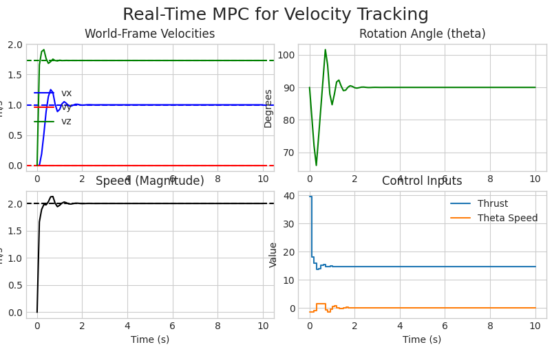
it is a simple 2D drone with a simplified dynamics (only gravity) the thrust is along the x axis and the x axis is pointinn upward at the start. I want to control the pitch (rotation around y) and the thrust to obtain a given speed in the x z plane. It compiles and runs but the result are very strange . I have spent a lot of time understanding what was wrong with various version of the code. You may run it as it is. You will see a pitch angle = PI/2 while achiving the desired velocity vector and having a thrust = hover thrust which is not possible but the solver found this solution ?
Code
from acados_template import AcadosOcp, AcadosOcpSolver, AcadosModel
from casadi import SX, vertcat, sin, cos, horzcat, Function
import numpy as np
import matplotlib.pyplot as plt
— Version Number for clarity —
VERSION = 36.1
— Define Global Constants —
G = 9.81 # Gravity (m/s^2)
M = 1.5 # Mass (kg)
U_ROT_AXIS = np.array([0.0, 1.0, 0.0]) # Pure Y-axis (pitch) rotation
def export_maneuver_model_world_frame():
“”"
Creates a self-contained AcadosModel for the target velocity maneuver.
- Dynamics are expressed in the WORLD frame.
- The drone’s orientation is described by an angle ‘theta’ around a fixed axis U.
“”"
model_name = “velocity_tracking_mpc”
x = SX.sym(‘x’, 4) # State: [vx, vy, vz, theta]
u = SX.sym(‘u’, 2) # Control: [Thrust, theta_speed]
p_param = SX.sym(‘p’, 3) # Parameters: [vx_ref, vy_ref, vz_ref]
vx, vy, vz, theta = x[0], x[1], x[2], x[3]
thrust, theta_speed = u[0], u[1]

# --- System Dynamics in World Frame ---
force_x_world = thrust * cos(theta)
force_y_world = 0
force_z_world = thrust * sin(theta)

dvx = force_x_world / M
dvy = force_y_world / M
dvz = (force_z_world - M * G) / M
dtheta = theta_speed
f_expl = vertcat(dvx, dvy, dvz, dtheta)

# --- EXTERNAL Cost Expression (Corrected) ---
velocity_error = x[:3] - p_param

# The cost ONLY penalizes velocity error and control effort.
# The pitch angle is now free for the controller to use as a tool.
W_vel = np.diag([100.0, 100.0, 100.0]) # High penalty for velocity error
R_ctrl = np.diag([0.01, 0.1])         # Penalty on control effort

cost_expr_stage = velocity_error.T @ W_vel @ velocity_error + u.T @ R_ctrl @ u
cost_expr_terminal = velocity_error.T @ W_vel @ velocity_error * 10

model = AcadosModel()
model.f_expl_expr = f_expl; model.x = x; model.u = u; model.p = p_param; model.name = model_name
model.cost_expr_ext_cost = cost_expr_stage; model.cost_expr_ext_cost_e = cost_expr_terminal
return model
def create_mpc_solver():
ocp = AcadosOcp(); model = export_maneuver_model_world_frame()
ocp.model = model
N = 20; Tf = 2.0 # Shorter horizon for MPC
ocp.solver_options.N_horizon = N
ocp.dims.nx = model.x.size()[0]; ocp.dims.nu = model.u.size()[0]; ocp.dims.np = model.p.size()[0]

ocp.cost.cost_type = 'EXTERNAL'; ocp.cost.cost_type_e = 'EXTERNAL'

# Set a minimum thrust to avoid freefall scenarios
ocp.constraints.lbu = np.array([M * G * 0.5, -np.pi / 2])
ocp.constraints.ubu = np.array([1000.0, np.pi / 2])
ocp.constraints.idxbu = np.arange(ocp.dims.nu)
ocp.parameter_values = np.zeros(ocp.dims.np)
ocp.constraints.x0 = np.array([0.0, 0.0, 0.0, 0.0])

ocp.solver_options.qp_solver = 'PARTIAL_CONDENSING_HPIPM'; ocp.solver_options.hessian_approx = 'GAUSS_NEWTON'
ocp.solver_options.integrator_type = 'ERK'; ocp.solver_options.nlp_solver_type = 'SQP'
ocp.solver_options.tf = Tf
ocp.solver_options.nlp_solver_max_iter = 100

json_file = 'acados_ocp_velocity_tracker.json'
acados_solver = AcadosOcpSolver(ocp, json_file=json_file)
return acados_solver
def main():
print(f"— Running Version {VERSION} —")
solver = create_mpc_solver()
model = export_maneuver_model_world_frame()
# Create a CasADi function for the dynamics for simulation
f_expl_fun = Function(‘f_expl_fun’, [model.x, model.u], [model.f_expl_expr])
sim_duration = 10.0; dt = 0.1; N_sim = int(sim_duration / dt)

# <<< CHANGE: Define Target Velocity using an angle and amplitude >>>
target_angle_rad = np.pi / 3  # 60 degrees from the horizontal
target_amplitude = 2.0        # m/s

# Calculate the target velocity vector from the angle and amplitude
# Note: This defines the direction in the X-Z plane.
target_velocity = target_amplitude * np.array([np.cos(target_angle_rad), 0, np.sin(target_angle_rad)])

# --- Start at rest in a hover orientation ---
x_current = np.array([0.0, 0.0, 0.0, np.pi / 2])

sim_x = np.zeros((N_sim + 1, 4)); sim_u = np.zeros((N_sim, 2))
sim_x[0, :] = x_current

print("Running real-time MPC for velocity tracking...")

# --- MPC Simulation Loop ---
for i in range(N_sim):
    # Set the reference (target velocity) for the entire prediction horizon
    for j in range(solver.N + 1):
        solver.set(j, "p", target_velocity)

    # Set the current state
    solver.set(0, "lbx", x_current)
    solver.set(0, "ubx", x_current)

    # Solve the OCP
    status = solver.solve()
    if status != 0:
        print(f'WARNING: solver returned status {status} at time step {i}.')

    # Get the optimal control input for the first step
    u_optimal = solver.get(0, "u")
    sim_u[i, :] = u_optimal

    # Simulate the system forward one step
    x_dot = f_expl_fun(x_current, u_optimal)
    x_current = x_current + dt * x_dot.full().flatten()
    sim_x[i+1, :] = x_current

print("Simulation finished.")

# --- Save Results to File ---
time_grid = np.linspace(0, sim_duration, N_sim + 1)
# The control inputs are one step shorter than the states, so pad with a zero row
sim_u_padded = np.vstack([sim_u, np.zeros((1, sim_u.shape[1]))])

# Create a version column as requested
version_col = np.full((N_sim + 1, 1), VERSION)

# Combine all data into a single array
results_data = np.hstack([
    version_col,
    time_grid.reshape(-1, 1),
    sim_x,
    sim_u_padded
])

header = f"Version, Time (s), vx, vy, vz, theta (rad), Thrust, theta_speed"
np.savetxt("simulation_results.txt", results_data, delimiter=", ", header=header, fmt='%.4f')
print("\nSimulation results saved to 'simulation_results.txt'")
# ---------------------------

# --- Plot Results ---
time_grid_u = np.linspace(0, sim_duration, N_sim)

plt.style.use('seaborn-v0_8-whitegrid')
fig, axs = plt.subplots(2, 2, figsize=(15, 10))
fig.suptitle('Real-Time MPC for Velocity Tracking', fontsize=18)

axs[0, 0].plot(time_grid, sim_x[:, 0], 'b-', label='vx'); axs[0, 0].axhline(y=target_velocity[0], color='b', linestyle='--')
axs[0, 0].plot(time_grid, sim_x[:, 1], 'r-', label='vy'); axs[0, 0].axhline(y=target_velocity[1], color='r', linestyle='--')
axs[0, 0].plot(time_grid, sim_x[:, 2], 'g-', label='vz'); axs[0, 0].axhline(y=target_velocity[2], color='g', linestyle='--')
axs[0, 0].set_title('World-Frame Velocities'); axs[0, 0].set_ylabel('m/s'); axs[0, 0].legend()

axs[0, 1].plot(time_grid, np.rad2deg(sim_x[:, 3]), 'g-')
axs[0, 1].set_title('Rotation Angle (theta)'); axs[0, 1].set_ylabel('Degrees')

axs[1, 0].plot(time_grid, np.linalg.norm(sim_x[:, :3], axis=1), 'k-')
axs[1, 0].axhline(y=np.linalg.norm(target_velocity), color='k', linestyle='--')
axs[1, 0].set_title('Speed (Magnitude)'); axs[1, 0].set_ylabel('m/s'); axs[1, 0].set_xlabel('Time (s)')

axs[1, 1].step(time_grid_u, sim_u[:, 0], where='post', label='Thrust'); axs[1, 1].step(time_grid_u, sim_u[:, 1], where='post', label='Theta Speed')
axs[1, 1].set_title('Control Inputs'); axs[1, 1].set_ylabel('Value'); axs[1, 1].legend(); axs[1, 1].set_xlabel('Time (s)')

for ax_row in axs:
    for ax in ax_row:
        ax.grid(True)
plt.tight_layout(rect=[0, 0.03, 1, 0.95])
plt.show()
if name == ‘main’:
main()
error message
I got no error message :
acados was compiled without OpenMP.
Running real-time MPC for velocity tracking…
Simulation finished.
Simulation results saved to ‘simulation_results.txt’
I hope someone can see what is the problem
Emmanuel