Hello everyone,
I am implementing Nonlinear Model Predictive Control (NMPC) for real-time trajectory tracking on my underwater vehicle using Acados and its Python interface. While the NMPC performed well in simulations, I am facing significant challenges in real-time experiments. The vehicle fails to track the reference trajectory, and the cost function does not behave as expected, despite extensive parameter tuning.
The core issues in my real-time experiments are:
- Poor trajectory tracking**: The vehicle does not follow the desired reference trajectory effectively, resulting in large steady-state errors.
- Unresponsive cost function**: The cost function shows minimal reaction to deviations from the reference trajectory, raising concerns about its role in optimization.
Key Observations:
*The control inputs vary but fail to generate meaningful corrections to the trajectory error.
- The system does not adapt well to changes in the reference trajectory, which was not an issue in simulations.
- Despite extensive variation of NMPC parameters (e.g., weights, prediction horizon, solver settings), the performance does not improve in real-time.
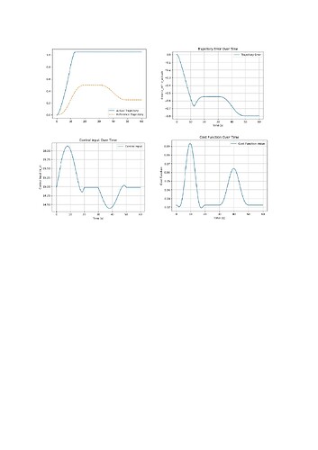
Attached is a figure showing the following results:
- Actual vs Reference Trajectory: The vehicle deviates significantly from the reference.
- Trajectory Error Over Time: Error remains large and does not converge.
- Control Input Over Time: Oscillations are observed, but they do not result in effective corrections.
- Cost Function Over Time: Minimal reaction, raising questions about solver performance.
Specific Questions:
- What strategies can I use to diagnose the unresponsiveness of the cost function in real-time experiments?
- Are there any specific tuning techniques or practical tips for NMPC parameters in real-time implementations?
- Could this be related to limitations of the Acados solver in real-time hardware conditions, and how can I address this?
I appreciate any insights or advice that could help resolve these issues. If you’ve encountered similar challenges in real-time NMPC implementations or have tips for debugging such problems, I’d be very grateful for your input. Thank you in advance!
***Code *****
Dynamics parameters
z, w = state[0], state[1]
tau_z = control[0]
m = 46.0 # Vehicle mass
d_z1 = 22 # Linear drag coefficient
d_z2 = 800 # Quadratic drag coefficient
F = 15 # Buoyancy force
Simplified dynamics
z_dot = w
drag = d_z1 * z_dot + d_z2 * z_dot**2
w_dot = (tau_z - drag * w - F) / m
state_dot = ca.vertcat(z_dot, w_dot)
CasADi dynamics function
f_dynamics = ca.Function(‘f_dynamics’, [state, control], [state_dot])
NMPC Configuration
ocp = AcadosOcp()
ocp.model.name = ‘depth_control’
ocp.model.x = state
ocp.model.u = control
ocp.model.f_expl_expr = state_dot
Prediction horizon
dt = 0.05
ocp.dims.N = 2 # Prediction steps
ocp.solver_options.tf = ocp.dims.N * dt
Cost function weights
Q = np.diag([1e12, 1000]) # Weights for [z, w]
R = np.array([[0.001]]) # Weight for tau_z
W = np.block([[Q, np.zeros((2, 1))], [np.zeros((1, 2)), R]])
ocp.cost.W = W
ocp.cost.cost_type = ‘LINEAR_LS’
ocp.cost.yref = np.zeros(3) # Reference for [z, w, tau_z]
ocp.constraints.lbu = np.array([-50.0]) # Lower bound for tau_z
ocp.constraints.ubu = np.array([50.0]) # Upper bound for tau_z
ocp.constraints.idxbu = np.arange(1)
def poly5_trajectory(t, t_start, t_end, z_start, z_end):
“”"
Generates a 5th-order polynomial trajectory.
“”"
T = t_end - t_start
if t < t_start:
return z_start, 0.0
elif t > t_end:
return z_end, 0.0
else:
a3 = 10 * (z_end - z_start) / T3
a4 = -15 * (z_end - z_start) / T4
a5 = 6 * (z_end - z_start) / T5
tau = t - t_start
z_t = z_start + a3 * tau3 + a4 * tau4 + a5 * tau5
w_t = 3 * a3 * tau2 + 4 * a4 * tau3 + 5 * a5 * tau**4
return z_t, w_t
Generate reference trajectories
z_trajectory, w_trajectory = ,
for t in time_array:
z_t, w_t = poly5_trajectory(t, 0, 20, 0, 0.5) # Example transition
z_trajectory.append(z_t)
w_trajectory.append(w_t)
Main Control Loop
while True:
try:
# Receive current state from robot
initial_state = np.array([ROV_z, ROV_w])
ocp_solver.set(0, ‘x’, initial_state)
    # Update reference trajectory
    for k in range(ocp.dims.N):
        ref_idx = min(global_idx + k, len(z_trajectory) - 1)
        yref_segment = np.array([z_trajectory[ref_idx], w_trajectory[ref_idx], 0.0])
        ocp_solver.set(k, 'yref', yref_segment)

    # Solve NMPC
    status = ocp_solver.solve()
    if status != 0:
        print(f"Solver failed at t={current_time:.2f}")
        break

    # Extract control input
    tau_z_optimal = ocp_solver.get(0, 'u')[0]
    control_inputs.append(tau_z_optimal)

    # Collect results
    actual_trajectory.append(ROV_z)
    trajectory_errors.append(z_trajectory[global_idx] - ROV_z)
    cost_function_values.append(ocp_solver.get_cost())

    # Update index
    global_idx += 1
    if global_idx >= len(z_trajectory):
        break

except Exception as e:
    print(f"Error: {e}")
    break
