I am working on a nonlinear MPC to achieve optimal raceline generation and following by using the model predictive contouring control (MPCC) formulation as stated in: https://arxiv.org/pdf/1711.07300 (at formula 13).
I found an implementation of this problem using acados in https://github.com/mlab-upenn/mpcc?tab=readme-ov-file but they linearize both the errors and the track around the previous solution of theta for that shooting node. Although this is a clever approach, I want to experiment with the results when not linearizing the problem.
I am using the python interface.
My first question is whether acados runs faster when using the nonlinear least squares cost formulation instead of an external cost formulation. I would think this is the case as the specific structure of a nonlinear least squares formulation can be exploited and solved more efficiently?
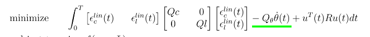
My second question is related to the linear term in the MPCC cost formulation (see figure). If I want to use the nonlinearLQ formulation, I can achieve this linear term by
Using the square root of the state theta_dot as nonlinear function and -Q_theta as diagonal element in the cost matrix W
Adding an extra state with constant value 1 to the states, such that a linear term is achieved by using nondiagonal elements in W hat couple theta_dot and 1.
A problem with this is that for both methods, the cost matrix W becomes non-positive-semi-definite and the nonlinearLQ requires W to be positive-semi-definite (PSD). My question thus is whether ACADOS will make it PSD by matrix manipulation such as adding a multiple of the unit matrix or will the solver always fail when the provided W matrix is not PSD?
In general, I would recommend to use the (non)linear least-squares cost module whenever possible. This allows you to use a Gauss-Newton Hessian approximation, which is often cheap to compute (compared to an exact Hessian) and guaranteed to be psd.
In your specific case with the additional linear term, you could
use an external cost formulation and in addition provide a custom Hessian corresponding to a Gauss-Newton Hessian with no contribution from the linear term, cf. this example for how to define a custom Hessian
use a convex-over-nonlinear cost formulation where the outer convex function is quadratic for the NLS terms and the identity function for the linear term, cf. this example and Section 3.5 of the problem formulation.
I’m not sure if you’re still actively working on this, but I wanted to share a suggestion regarding the NLS formulation that might help. I’ve run into similar issues myself.
Instead of ensuring track progress by using that negative linear term, an alternative approach is to introduce a quadratic penalty on the difference between the projected velocity (the virtual input) and a reference velocity. This reference velocity you can choose yourself or let a planner do for you. But this way your cost can be written into NLS form and you can safely use the Gauss-Newton Hessian approximation. This will yield far more stable results than the exact Hessian approach from my experience.
If you’re working on racing scenarios where the track is fixed and doesn’t have to be updated at runtime, CasADi’s interpolant function can also be very useful. It allows you to differentiate through lookup tables, which is nice for incorporating precomputed reference trajectories. Note that this requires you to use CasADi MX types instead of SX. Use them for your dynamic/kinematic model and for the track progress variable. Lastly for this to work with the Acados setup, make sure to set constraint types to ‘BGH’.